The FILTER function replicates and extends Excel AutoFilter filtering functionality in formula form.
The FILTER function allows us to filter a range of data based on defined criteria.
By default, the FILTER function will return multiple values, which will be placed in the neighboring cells (to the bottom and/or to the right). I.e., we are dealing with dynamic array formulas here.
The syntax of the FILTER function is as follows:
= FILTER ( array ; include ; [if_empty] )
The (return) array represents an array or a range of cells to return values from.
The include part of the argument typically consists of the corresponding array and filtering criteria defined for that corresponding array. Criteria are defined using the following Comparison operators:
equal to =
greater than >
greater than or equal to >=
less than <
less than or equal to <=
not equal to <>
The OR logic can be applied by using the addition operator + and/or the AND logic can be applied by using the multiplication operator *.
We can perform simple vertical filtering in the following way:
Here, we are selecting rows from the cell range D2:I9.
Only the rows where corresponding rows in the cell range A2:A9 contain text equal to green are included.
Note, the FILTER function does not support partial matches!
A formula such as =FILTER(D2:I9;A2:A9=”g*”) would return a #CALC! error.
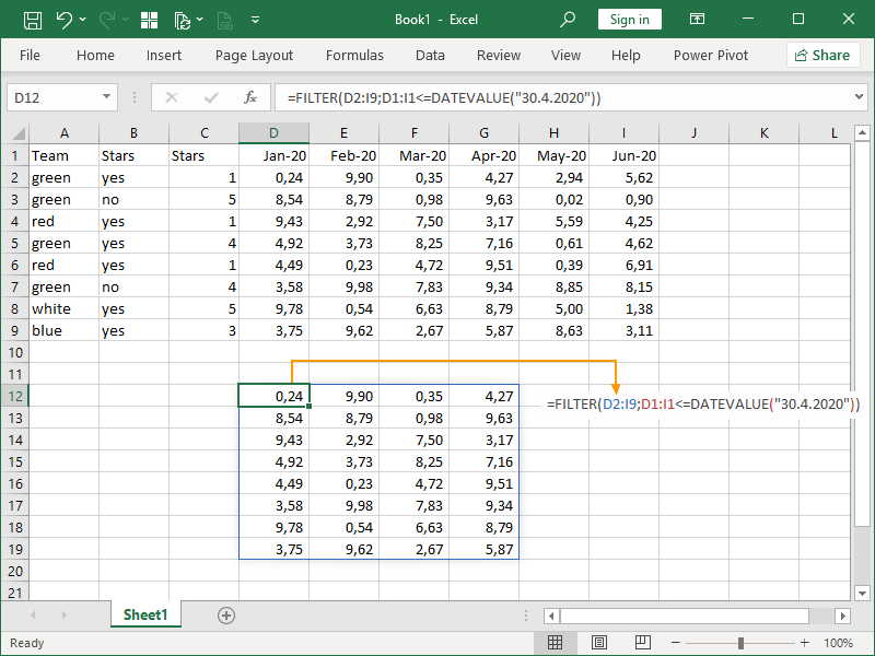
We can perform simple horizontal filtering in the following way:
Here, we are selecting columns from the cell range D2:I9.
Only the columns where the corresponding columns in the cell range D1:I1 contain a date value less than or equal to are included.
Note, we’ve nested a rather simple function as filter criteria!
Not only simple functions but also complex calculations can be nested as filter criteria. If needed, those formulas can be enclosed in parentheses ().
We can apply both vertical and horizontal filters at the same time by nesting one FILTER function inside another FILTER function:
Here, we are first selecting rows from the cell range D2:I9 for which corresponding rows in the cell range A2:A9 contain text equal to green.
We are using that return as an array part of the argument for the second FILTER function, where we are selecting columns for which corresponding columns contain a date value less than or equal to 30.4.2020.
The order of filtering is irrelevant here; we could also first filter the desired columns and then filter the desired rows.
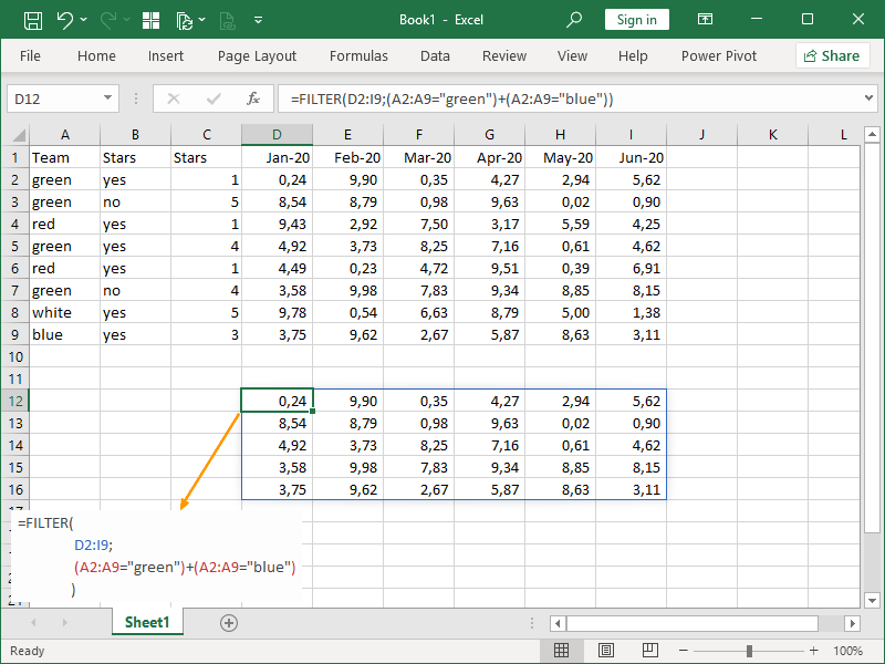
We can use the addition operator + to filter rows containing text equal to green OR containing text equal to blue:
Note, different filters are enclosed in parentheses ().
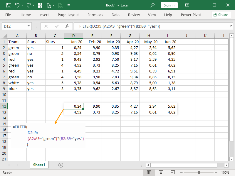
We can use the multiplication operator * to filter rows containing text equal to green in the first corresponding array AND containing text yes in the second corresponding array:
Note, different filters are again enclosed in parentheses ().
Multiple OR and AND criteria can be freely combined:
Here, we are first selecting columns from the cell range D2:I9, which contain data for the period 01.01.2020 to 31.03.2023.
We are using that return as an array part of the argument for the second FILTER function, where we are selecting rows that, in corresponding arrays, contain green OR blue in the first array, AND there are no blanks in the second array (i.e., we are filtering out blank cells), AND stars are greater than or equal to 3 in the third array.
Note the usage of parentheses ().
What is going on here from a technical standpoint?
Every time we apply a filtering criterion to a corresponding array using a comparison operator, a new array is calculated that contains TRUE and FALSE values.
When we add or multiply those arrays, as TRUE is the same as 1 and FALSE is the same as 0, we will generate new arrays that will contain the results of those additions and multiplications.
In mathematics, multiplication is performed before addition in order of operations, and without the use of parentheses (), our criteria would not be properly applied.
Also note, we don’t even actually have to define criteria as shown in our examples. What we actually need are corresponding arrays that contain TURE and FALSE values; we can generate them in any way.
It can be of little use to filter some numbers without context.
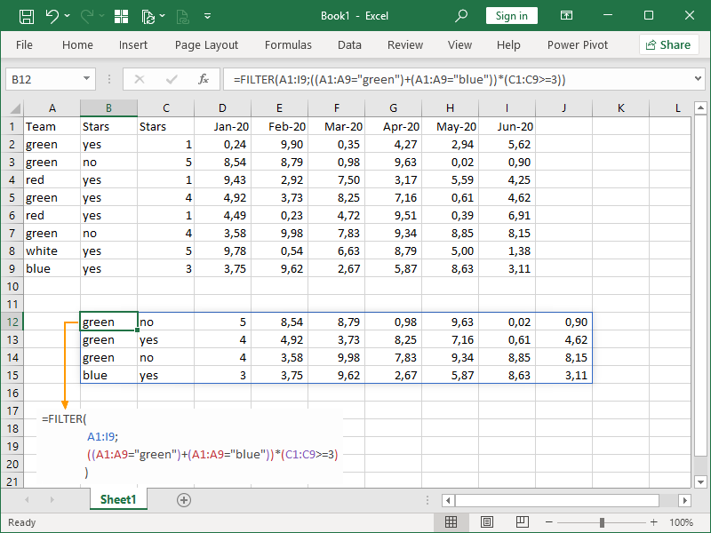
In principle, we can add headers or columns to the left of the values by expanding our return array:
In this example, we’ve used the whole table, cell range A1:I9, as our return array.
This is not ideal. We have no headers, and we have no control over which columns to the left will be returned.
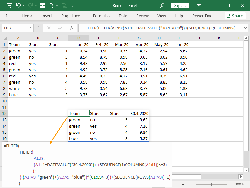
However, we can also add both headers and columns to the left of the values by defining additional filtering criteria:
Here, we are first selecting columns from the cell range D2:I9, which contain data for the date 30.04.2023. We are using that return as an array part of the argument for the second FILTER function, where we are selecting rows that, in corresponding arrays, contain green OR blue in the first array, AND stars that are greater than or equal to 3 in the third array.
In both of the used FILTER functions, we are combining the SEQUENCE function with the ROWS or the COLUMNS function in order to generate an additional array, using which we can add the first three columns and the top row to the return of the FILTER function.
Again, given the importance of the order of operations, note the usage of parentheses ().
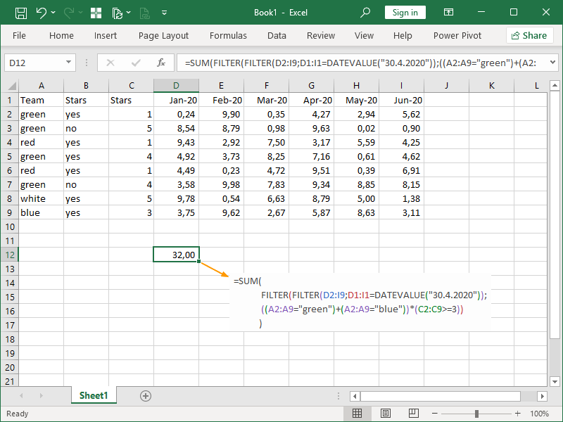
We can also nest the returns of the FILTER function into other functions:
Here, we are nesting the return of the FILTER function into the SUM function, basically replicating the functionality of the SUMPRODUCT function.
However, the possibilities are practically endless.
We can nest the return of the FILTER function into the COUNT, AVERAGE, MIN or MAX functions.
We can nest the return of the FILTER function into the INDEX function in order to lookup the 2nd, the 3rd, or the nth value.
We can nest the return of the FILTER function into the SUMIFS function as the sum range, or use other IFS functions for related purposes.
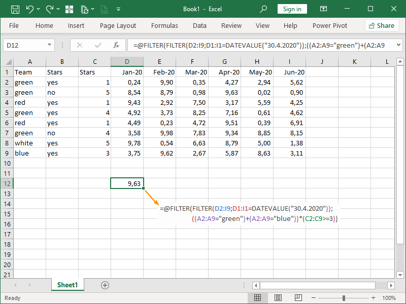
We can use the implicit intersection operator @ in order to return only the first filtered value, thus changing the default behavior of the FILTER function:
Optional if_empty part of the argument contains an alternative value, to be returned if the filter returns nothing:
Here, we tried to filter rows with blank cells in the cell range B2:B9.
As there are no such rows, a #CALC! error would be returned by the function.
However, we’ve specified zero as the default return in the if_empty part of the argument, so zero is returned.
One final note: both workbooks have to be open if you are filtering from a different workbook.
Dig deeper:





15 thoughts on “FILTER function”