Spreadsheet basics

Starting with spreadsheets

Spreadsheets are used to store and manipulate data.

That data is stored in cells and organized in tables (i.e., rows and columns).

Table cells can contain a value (text or number) or a formula.

Formulas calculate new values, usually by referencing existing values.

Both values and formulas can be easily modified.

 

These simple concepts can then be used to perform basic tasks, i.e., you can use your spreadsheet as a tape calculator.

On the other hand, the strength and scalability of the spreadsheet concept enables ordinary users without programming knowledge to, basically, create and manage rational databases and write programs.

 

This is what an empty spreadsheet looks like in Microsoft Excel:

You are now on cell A1, as indicated by the highlighted border around cell A1.

A1 is the address of your cell, i.e., your cell is located in column A of XFD columns and row 1 of 1048476 rows.

 

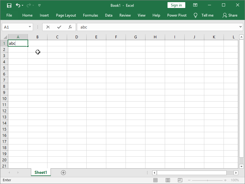
Think of a cell as a container for some of your data. If you want to add something to cell A1 or change existing data, you can enter it into the cell by double-clicking it.

You can type some text in that cell. If you do, it will be aligned to the left.

 

You can also type a number in that cell. If you do, it will be aligned to the right.

You can also do this by typing in the formula bar. You can change the address of the cell you are editing on the left of the formula bar, and edit the contents of your cell on the right of the formula bar:

 

You can select multiple cells at once. If you right-click on your selection, you will get a pop-up menu with options to manipulate all those cells at the same time. For example, you can delete the contents of all selected cells.

You can select one whole column if you left-click column name. If you click on column name A, you will select column A. If you click on column name A and drag right, you will be able to select multiple columns at once:

It works the same way with rows.

 

The width of your columns and the height of your rows are irrelevant for your data; they’re purely visual. If you want to change the width of column A, position your mouse between the names of columns A and B, click, and drag. You can change row height the same way.

 

This array of cells organized in rows 1 of 1048476 and columns A to XFD is called a spreadsheet, worksheet, or just sheet. Here, it’s called “Sheet1”, but we can also rename it after we double-click it:

 

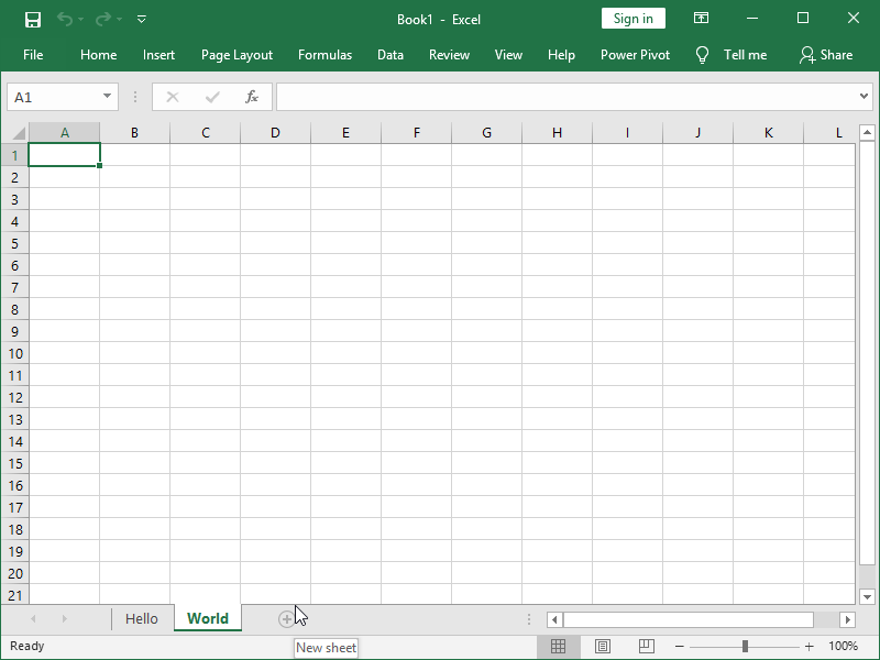
By clicking the “New sheet” button, you can also add new sheets:

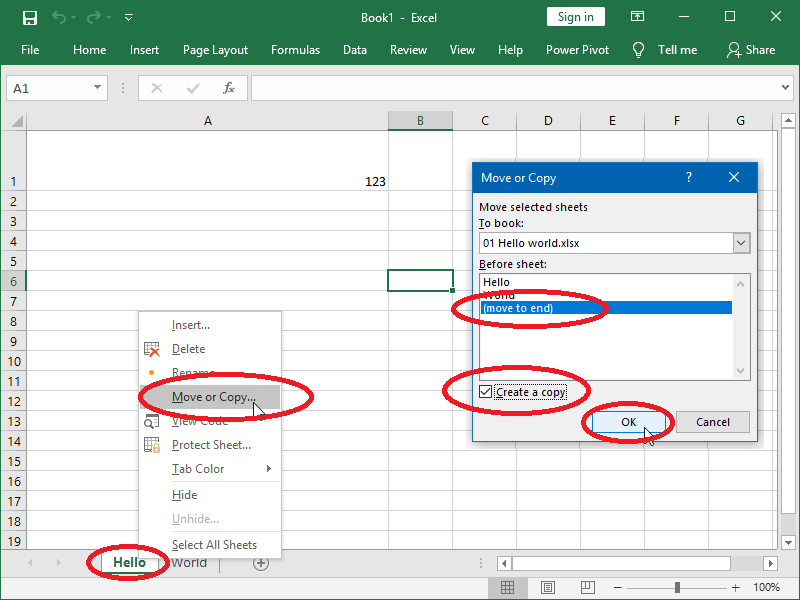
If we wanted to do so, we could also duplicate any existing sheet by right-clicking its name and selecting “Move or Copy…”:

 

One or more of these sheets combined are called a workbook, or just a book.

You can already see at the top center of the window that your workbook was automatically named “Book1”. You can rename your workbook by saving it with the save button located at the top left of the window:

We have now named our workbook “01 Hello world”. Excel workbooks should be saved with the file extension “.xlsx”.

Note that Excel can open, read, and save files with many different types of extensions, such as legacy spreadsheets with the extension “.xls”, spreadsheets of other programs such as LibreOffice with the extension “.ods”, web pages, comma-separated values and text files. Nevertheless, in order to avoid issues, it’s recommended that you save any file you create or modify with Microsoft Excel as “.xlsx”.

 

How to use formulas in Excel?

A table cell can contain a value (text or number) or a formula.

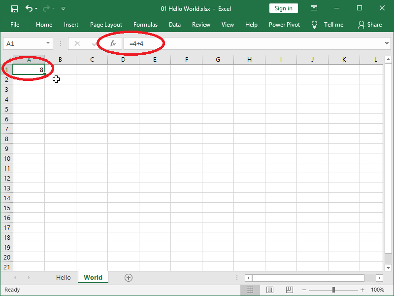
If a cell contains a formula, it actually contains both that formula and a value calculated by that formula. While we are on a cell, we will see that calculated value. In the formula bar, we will see the formula for that cell. Here is how that looks:

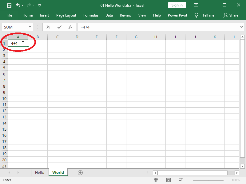
But if we double-click on the cell and enter it, we will also be able to see and change the formula. Here is how that looks:

 

We can also refer to another cell with the formula, including empty cells, and those will be interpreted as zero.

The referred cell doesn’t have to be on the same sheet. For example, in order to refer to cell A1 in sheet “Hello” we have to first invoke the name of that sheet followed by an exclamation mark ! and then the cell address:

 

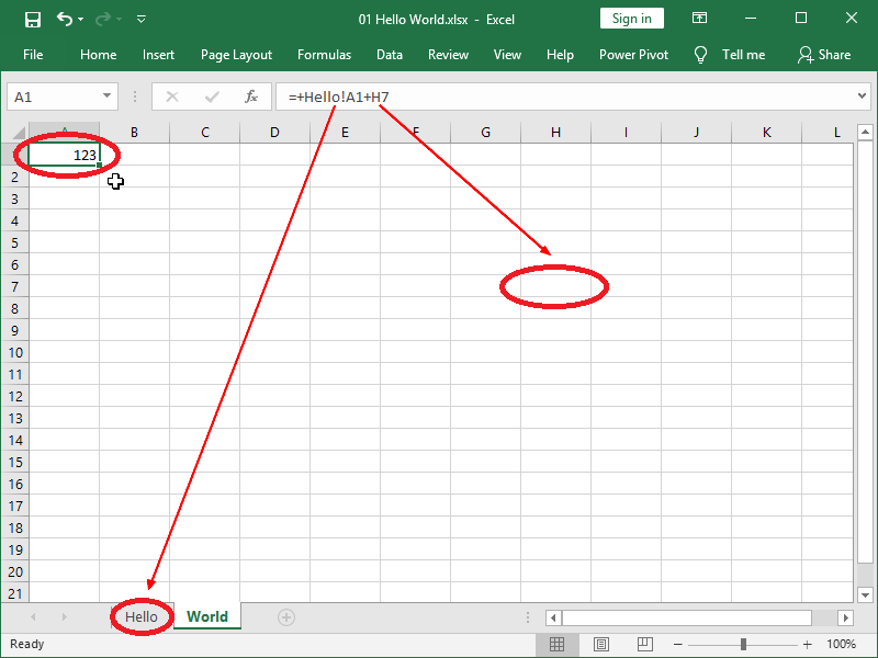
We can start writing any formula by writing an equals sign = or even a plus sign +, with Excel automatically adding an equals sign in that case.

Formulas can contain:

• a value,
• the address of a cell (a value stored in the cell we are calling),
• a function,
• any combination of the above.

Basic mathematical operations we can perform with values are addition + subtraction –, multiplication *, division / and exponentiation ^.

 

When editing formulas directly in the cell, Excel automatically highlights referenced cells visible on screen:

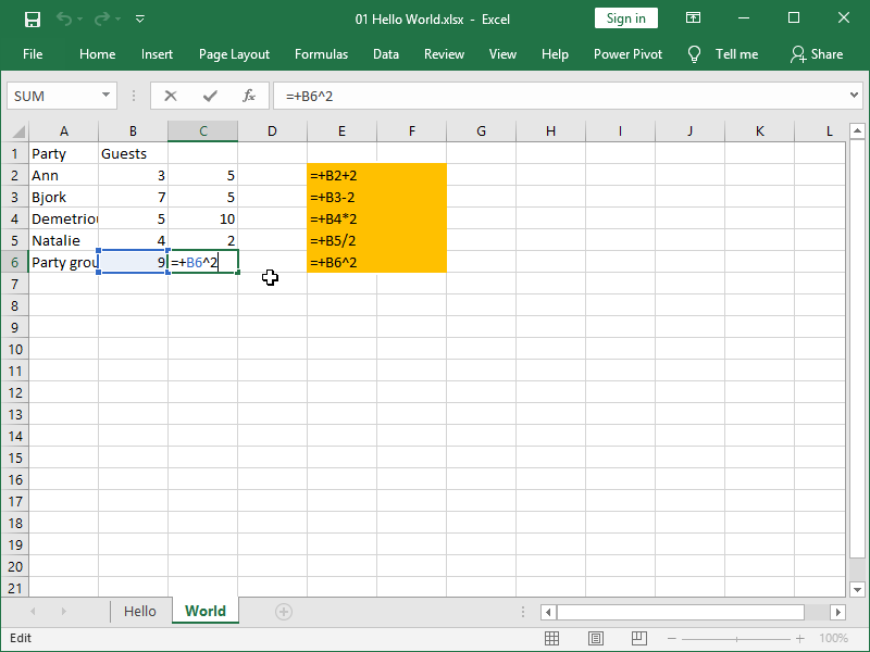
Here, we were referring to the values in cells in column B and performing different mathematical operations on them with normal or relative references.

 

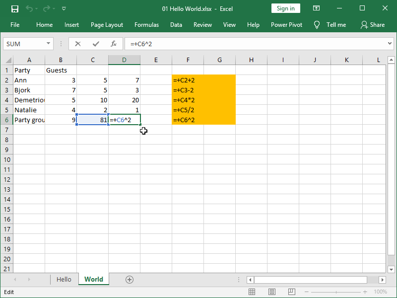
If we copy or drag the formulas containing relative references, for example, if we copy formulas from column C to column D, the cells referred to will also move.

 

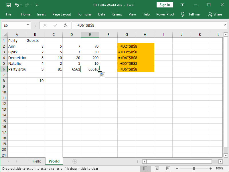
If we want to avoid that, we can use locked or absolute references. That type of reference, in addition to column and row addresses, also contains dollar signs $:

Even if we now drag that formula down, we will still refer to cell B8 in all of the new formulas:

We are also able to lock only the column we are referring to by placing a dollar sign in front of a column reference but not a row reference, i.e., if we write $B8. This works the other way too, i.e., we can write B$8.

The dollar sign has no effect on calculations themselves, and absolute references are in principle only useful if we are copying or dragging formulas and want to ensure that the same cell, column, or row is always referenced.

 

How to use functions in Excel?

In addition to the basic mathematical operations, we can also use a huge number of functions available in Excel in our formulas.

You can see a complete list of those functions under Formulas > Insert Function, together with a short description of each function:

 

Alternatively, if you insert the function by directly typing its name in the cell, you also get some help from Excel:

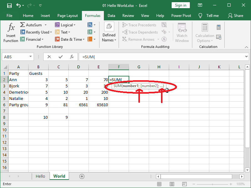
Here you can see that, in this example of the SUM function:

• the function should be called by name with arguments between parenthesis, i.e., SUM ()
• you can aggregate however many numbers you desire, as indicated by three dots …
• depending on your location, the different numbers you are aggregating should be separated by a colon , or a semicolon ;.

 

In functions, you can also:

• reference cells
• reference ranges of cells
• call other functions.

As mentioned before, you can also combine any number of functions, cell references, and numbers in formulas.

Here is one example of all of those principles:

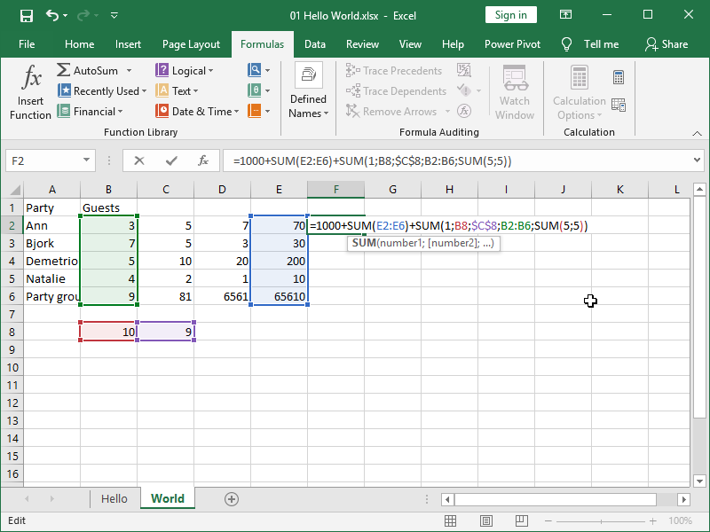
As you can see, Excel also helpfully highlights cell ranges the same way it does for the cells you are referring to.

The purpose of a function is to make your life easier, i.e., it is easier and less prone to errors to write a formula such as =SUM(E2:E6) than a formula such as =E2+E3+E4+E5+E6.