
How to insert or remove a filter
Excel AutoFilter features enable us to quickly sort and filter, i.e., to quickly order, select from based on a criterion, or analyze tabular data.
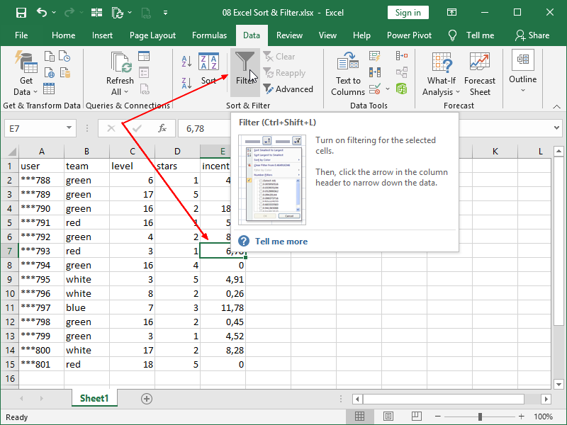
Feature is available under both Home and Data ribbons, as Sort & Filter:

We can insert a filter by positioning ourselves in any cell that is a part of a table and using the Filter button:
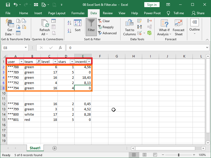
This is what a table with an inserted filter looks like:

Marked with red, headers have drop-down arrows that can be used to filter the data.
Marked with orange is the data; note that the filter extends only to the end of row 15, no further.
This is what our worksheet will look like if we, for example, filter only green team members:

In cell B1, we will see an indicator that something is filtered in that column.
On the left, we will see an indicator that some rows are not visible, i.e., not filtered.
We will not see the data contained in filtered-out parts of our table, and we will also not see the data in the columns outside of the filter scope!
For example, if we had some data in the G5 cell, it would also not be visible, as the whole rows are hidden when we filter out something.
However, we will encounter issues if we try to filter non-continuous data such as this:

If we just position ourselves in any cell that is a part of a table and use the Filter button in order to insert a filter, Excel will not necessarily recognize all the contents we are trying to filter:
In order to properly filter this data set, we should first select all of the data we are trying to filter, and only then select the Filter button:

Only in that case, even the non-continuous data will be filtered properly:

Also, consider this example. You have continuous data in rows, but the data in your columns is non-continuous. The easiest way to properly insert a filter here is to select the whole first row and then select the Filter button:

In that case, all of the columns containing data, and also columns in-between columns containing data, will be selected in the filter:

However, note that now again not all of the rows are selected; the data in cell K16 is outside the filter scope, as Excel (in)correctly interpreted our intention as selecting the cells in the range A1:K15. If we want to include the cell K16 in the filter, we will have to insert a filter while having the cells in the range A1:K16 selected.
We can both clear and remove filter completely by pressing the Filter button again:

On the other hand, the Clear button will only remove our present selection of slicers; the filter will still remain without the need to insert it again.
The Reapply button will refresh the filter based on the data currently in the table; for example, had we modified our data by changing the value in the B2 cell to red, the rows filtered would not update automatically to hide row 2.
Also note the behavior of filters with filtered-out rows.
Let’s say you want to delete rows you’ve filtered. You can select all or some of the visible rows and delete them; rows that are filtered-out will not be affected.
Let’s say you want to delete the data in some or all visible cells. You can select those cells and press Delete. Cells that are filtered-out will not be affected.
Let’s say you want to copy only data that is visible. You can select, copy, and paste that data; rows and cells that are filtered-out will not be copied.
This is, for example, what it would look like if we’d deleted all of the filtered rows from our previous table and then cleared the filter:

This is the expected behavior of the Filter feature.
However, in some cases, this will not happen, and hidden rows and cells will be deleted, cleared, or copied.
Select Visible Cells, here visible on the Quick Access Toolbar, will help in some of those cases by forcing Excel to actually select only visible cells.
Filtering in Excel
Now consider the following example:

In this filter, headers are highlighted red, columns containing text are highlighted orange, and columns containing numbers are highlighted yellow.
Some of the data, i.e., team and star columns, is also color-coded.
We will usually filter data with the help of the main filter window located under Search:

In this example, as the team column has a filter applied, it will be showing an appropriate indicator.
As green is filtered, it will have a checkmark.
As only green is filtered, Select All will not have a checkmark but will rather just indicate that something is filtered.
As blue, red, and white are filtered-out, they will not have a checkmark.
We can add blue, red, or white to the filter by adding checkmarks to them.
We can also remove filtering by adding checkmarks to all options, i.e., green, blue, red, and white, or by using the Clear Filter From option.
The Search option is useful when dealing with a large number of different unique values in rows. When we use the Search field, search results will be shown in the same area:
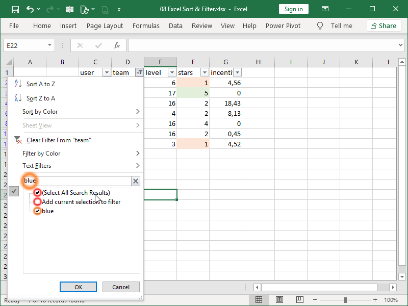
Two new options will now appear.
Select All Search Results will be automatically selected, but it can be unselected, and only individual search results selected.
Add current selection to filter will not be automatically selected; in this example, in order to filter both green and blue rows, we would have to select it manually.
Custom filters will enable us to have even greater control over filtering:

Custom AutoFilter enables us to filter data based on two criteria, with both And and Or logic available.
These are the Comparison operators available:
- equals,
- does not equal,
- is greater than,
- is greater than or equal to,
- is less than,
- is less than or equal to,
- begins with,
- does not begin with,
- ends with,
- does not end with,
- contains,
- does not contain.
Shortcuts to some of those are already available in the Text Filters menu, as visible with menu items prior to Custom Filter.
Wildcard characters are also supported, and you can:
- use question mark ? to represent any single character, i.e. g?een will filter green,
- use asterisk * to represent any series of characters, i.e., gr*n will filter green,
- use tilde ~ followed by a question mark ?, asterisk *, or tilde ~ in order to filter actual question marks, asterisks, and tildes.
When filtering numbers instead of text, under Number Filters, we will have several additional interesting options available:
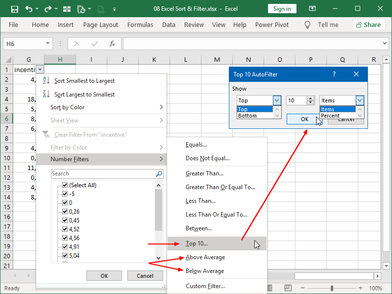
Above Average and Below Average will enable us to filter items above and below average, respectively.
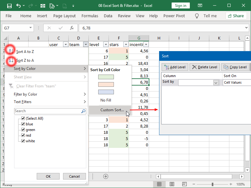
Filter by Color will enable us to filter our data by cell color:

Colors used in the table rows will be offered, as well as the No Fill option for not-colored cells.
Naturally, this option will only be useful if our data is already properly color-coded.
Some not-so-common filtering options are also available by right-clicking on the data inside a filter. For example, by right-clicking on the F4 cell and selecting the Filter option in the menu, the following options will become available:

Filter by Selected Cell’s Value will filter-our all rows with a value different than the cell that was right clicked on.
Filter by Selected Cell’s Color, Filter by Selected Cell’s Font Color and Filter by Selected Cell’s Icon will do the same with the various types of formatting available for the cell.
Filters themselves can be active on multiple columns at once, and the order in which they are applied or removed is irrelevant.
All of the filters can be removed by clicking the Clear command on the ribbon.
Filter from the individual column can be removed by clicking the Clear Filter From “column_name” command in the drop-down menu.
Marked red are the positions of those commands in the following example:

Sorting in Excel
Sorting in Excel relates to sorting the data
- from smallest to largest values (ascending order of numbers, oldest to newest date, A to Z),
- or from largest to smallest values (descending order of numbers, newest to oldest date, Z to A),
- according to color,
- according to Custom Lists.
When numbers and text are contained in the same column, the column can still be sorted. Text values will be treated as “larger” than numbers.
Numbers formatted as text will be treated as “smaller” than actual text but “larger” than actual numbers. Date and/or time mixed with other kinds of data will be treated as numbers, i.e., sorted by underlying decimal number behind the date.
When sorting according to color, the starting sorting order is automatically generated by the first appearance rule, and it can be rearranged.
Custom Lists are an advanced option that can be generated by the user at will under Custom Sort.
While sorting is always available in filtering menus, it is not strictly related to filtering, and there are important differences.
Most important is that, unlike filtering, sorting is permanent.
There is no such thing as a Clear Sort button; sorting is permanent, barring the use of the Undo button.
Next, we will show how to sort data without filtering.
That can be accomplished simply by positioning ourselves somewhere in the column we want to sort our data by, for example, cell D10, and then using the Sort A to Z command:

Another option is to right-click that (or any other cell) and then select the same option in the Sort menu:
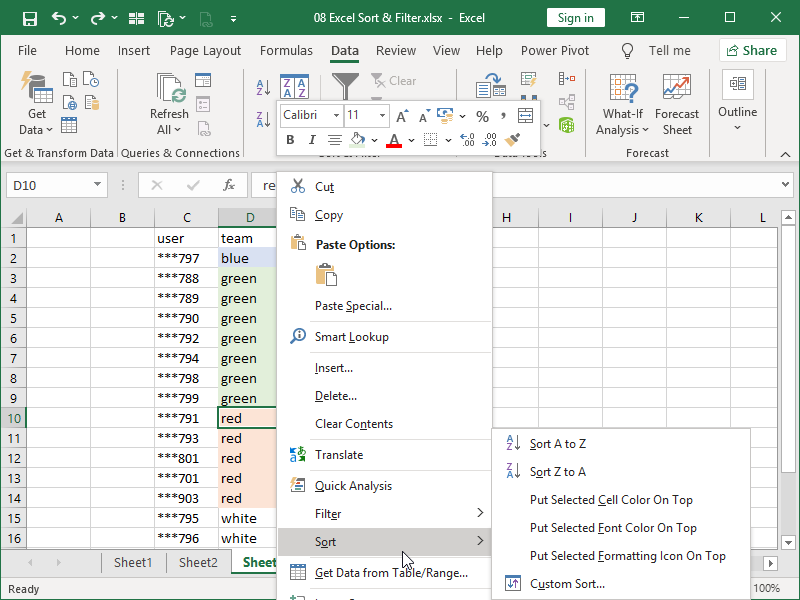
That menu also contains some additional options, such as Put Selected Cell Color On Top, Put Selected Font Color On Top, and Put Selected Formatting Icon On Top.
By selecting, for example, Put Selected Cell Color On Top, we can move rows marked with red on top without affecting the rest of the sorting order, with the end result looking like this:

In contrast with filtering, the order in which sorting is applied is relevant.
Consider the following example, we’ve additionally sorted our table by “stars” column, from largest to smallest:

The first rows all contain 5-star user ratings, but inside that subgroup, items are still sorted as they were before, i.e., first are red team users, then blue team users, then green team users, and at the end white team users. The same applies for sorting inside all subgroups of user ratings.
The Custom Sort or Sort window will offer all the available and some additional sorting options in one place. It can be activated both from the ribbon and from the right-click menu, as well as from the filter drop-down menus.
In the following example, we will activate it by positioning ourselves in the D2 cell and selecting Sort button on the ribbon:

Note that when the Sort window is activated, cells that are being sorted are highlighted in the background.
My data has headers checkbox can be used to expand our sort area to row 1, but this is not necessary as our first row indeed does contain headers, which were automatically detected.
We can also right away set up multiple sorting commands with the help of Add Level.
Levels and results of one such sorting are shown here:
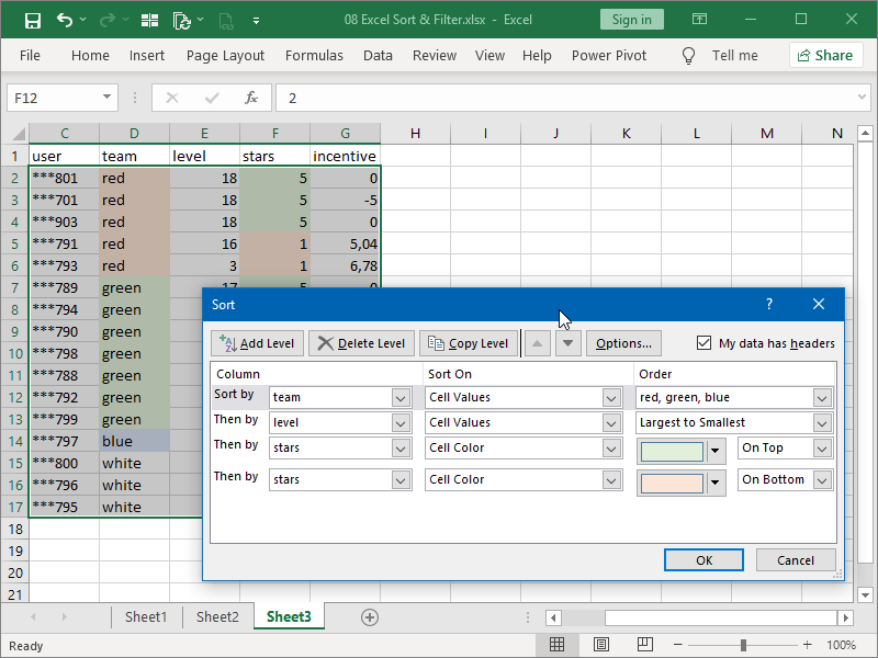
The first thing to note here is that Custom Sort is actually remembered by Excel; while starting sorting can’t be restored without the Undo button, settings here can be modified without having to be replicated from the start. Also, the order in which the columns are sorted is the reverse of what we would have to do in order to manually achieve this result!
Next, note the order in which the team column is sorted; that order is something called Custom List which can be created, modified, and saved for later in the Order drop-down menu.
Finally, even though sorting is not necessarily related to filtering, it is available in all of the filter drop-down menus and is usually used in combination with filters.
Indicators that sorting was performed in those filters will also be visible:

This data was sorted with the help of the Custom Sort, first from smallest to largest values based on the incentive column (note the indicator in the G1 cell), and then according to the custom list based on the team column (note the indicator in the D1 cell).
Had we sorted the data manually, without Custom Sort, only the last used sorting indicator would be visible, and not both.
Visible filters can be cleared and removed, and with that happening, filtered-out rows will then be shown, but the sorting will remain!
Sort & Filter functions
Modern iterations of Excel offer several functions that can be used to filter and sort data.
The FILTER function allows us to filter a range of data based on defined criteria.
The UNIQUE function allows us to return a list of unique values in a list or range.
For related Excel’s built-in feature, Remove Duplicates, see here.
9 thoughts on “Sort & Filter in Excel”