Combining SUMIFS with INDEX MATCH

Using the SUMIFS function, we can sum all of the values in a defined column (or row) that meet one or more criteria.

When SUMIFS is combined with INDEX MATCH, that sum range doesn’t have to be defined anymore; it is now rather specified in the function arguments.

By combining SUMIFS with INDEX MATCH, we can then sum all of the values that meet multiple criteria in different rows and columns and do this in a simple way, avoiding complex and resource-intensive array formulas.

 

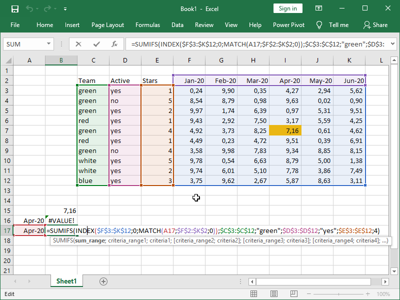
Let’s look at this table:

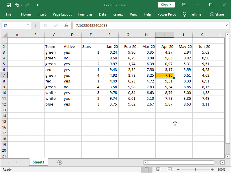
Let’s say we want to retrieve the value in the I6 column (marked orange).

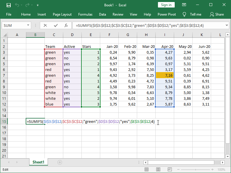
With the SUMIFS formula, that is rather simple:

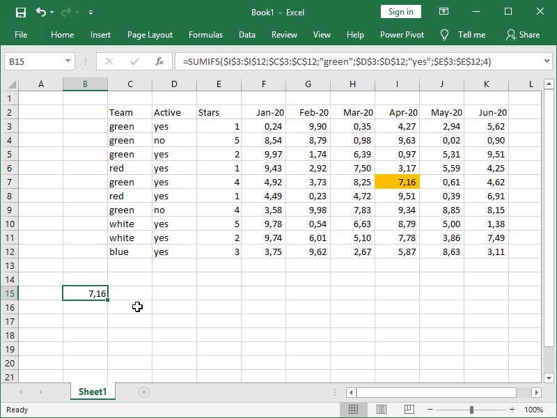
We’ve successfully retrieved our value:

 

However, we don’t always want to retrieve data from just the Apr-20 column; we want to retrieve data from the specified column. Here is where INDEX MATCH comes into play. With INDEX MATCH, we can retrieve the specified column, which we will later use as sum_range in the SUMIFS formula.

If we specify row number as 0, all of the rows, i.e., the whole column, will be returned:

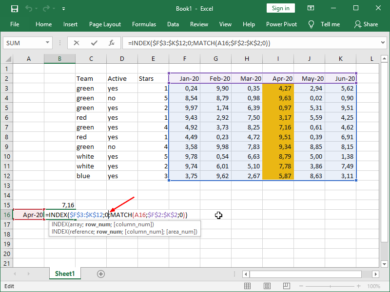
This by itself doesn’t produce anything useful, as we are returning the whole column into a single cell:

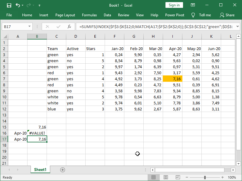
Only once we combine the formulas, i.e., the column returned by INDEX MATCH is our sum_range in the SUMIFS formula, we can return our number for the specified column:

We’ve now successfully retrieved our value from the specified column, for the specified criteria:

 

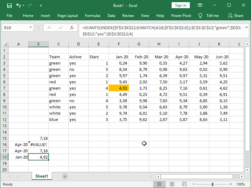
We can use the exact same formula to retrieve our value from any column that we want:

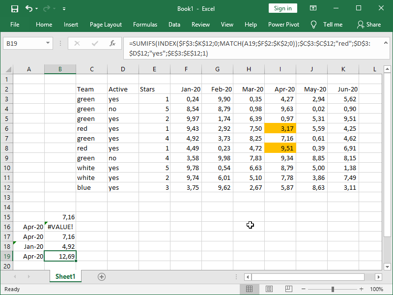
Naturally, if our criteria are matched in multiple rows, we will return the sum of those returns with the SUMIFS formula:

 

The basic principles shown here can be applied to other formulas as well. For example, you can combine COUNTIFS, AVERAGEIFS, MINIFS, MAXIFS, or even legacy functions such as SUMIF with INDEX MATCH.

All you have to do in order for your formulas to work properly is:

• define your row number as zero in INDEX MATCH in order to return the whole column
• make sure that your column is of the same size and in the same position as your criteria columns.

 

If we were to combine SUMIFS with INDEX MATCH in order to retrieve data from an Excel Table using structured references, the last formula shown above would look like this:

=SUMIFS(

INDEX(Table[[Jan-20]:[Jun-20]];0;MATCH(TEXT(A15;”[$-en-US]MMM-YY”);Table[[#Headers];[Jan-20]:[Jun-20]];0));

Table[[Team]:[Team]];“red”;Table[[Stars]:[Stars]];“yes”;Table[[Stars2]:[Stars2]];1)

This formula is easier to understand, but at the same time, special considerations have to be given to the numbers formatted as text in column names.

 

Are you looking for a way to sum values based on outside criteria? You can nest INDEX MATCH as your SUMIFS criteria.

If you prefer the XLOOKUP function to the INDEX MATCH combination, see how to combine SUMIFS with XLOOKUP in order to sum all of the values that meet multiple criteria in different rows and columns.

Need even more power? See how to combine FILTER with INDEX MATCH in order to return values based on criteria that are not present in the table we are returning values from.

 

Dig deeper:

Conditional calculations

Lookup with unique identifiers

Lookup with multiple criteria

Combining SUMIFS with XLOOKUP