We can use the INDEX function to designate a cell range (array) from which we want to retrieve data and, at the same time, use the MATCH function to specify the address of a cell in that cell range (array), i.e., row and column.
The MATCH function returns the relative position of the item in the range, either a row or a column.
The relative position is returned in the form of an integer number, such as 1, 2, 3,…
The syntax of the MATCH function is as follows:
= MATCH ( lookup_value; lookup_array; match_type)
The lookup value can be either a text or a number, inputted directly into the function or as a cell reference.
When looking up numbers, other than match type 0, exact match, we can also use the following types of matches:
- 1, less than or equal to match, finds the largest value that is less than or equal to the lookup value, while the lookup array must be placed in ascending order (from smallest to largest numbers, oldest to newest date),
- -1, greater than or equal to match, finds the smallest value that is greater than or equal to the lookup value, while the lookup array must be placed in descending order (from largest to smallest numbers, newest to oldest date).
Given the requirement that the lookup array must be sorted in ascending or descending order, in principle, we should manually sort those arrays beforehand.
In modern versions of Excel, we can also use the SORTBY function to sort our arrays.
However, if we have the SORTBY function available, we will also have the updated version of the MATCH function available, the XMATCH function. In contrast with the MATCH function, there are no requirements for the data to be presorted in ascending or descending order with the XMATCH, resulting in a cleaner code.
The XMATCH function also returns the relative position of the item in the range, either a row or a column.
The relative position is returned in the form of an integer number, such as 1, 2, 3,
The syntax of the MATCH function is as follows:
= XMATCH ( lookup_value; lookup_array; match_mode; search_mode)
The lookup value can be either a text or a number, inputted directly into the function or as a cell reference.
When looking up numbers, other than match type 0, exact match, we can also use the following types of matches:
- -1, exact match or next smaller item, finds the largest value that is less than or equal to the lookup value,
- 1, exact match or next larger item, finds the smallest value that is greater than or equal to the lookup value,
- 2, wildcard character match.
Note how match types here are the same as in the XLOOKUP function, exactly opposite of the MATCH function.
Consider the following example:
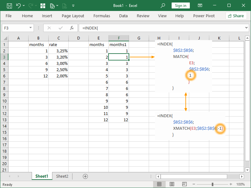
In column B, we have several months, and in column C, related interest rates.
We need to interpolate rates for the missing months. The rate for the 2nd month will be interpolated based on the rates for the 1st and 3rd months, etc.
In column E, we have a list of the next 12 months.
We can use match type 1 (less than or equal to) in order to retrieve the first smaller value than the one we are looking up.
Our lookup array ($B$2:$B$6) is already sorted from smallest to largest, so no additional sorting is needed:
With the XMATCH function, we are using match type 1 (exact match or next smaller item).
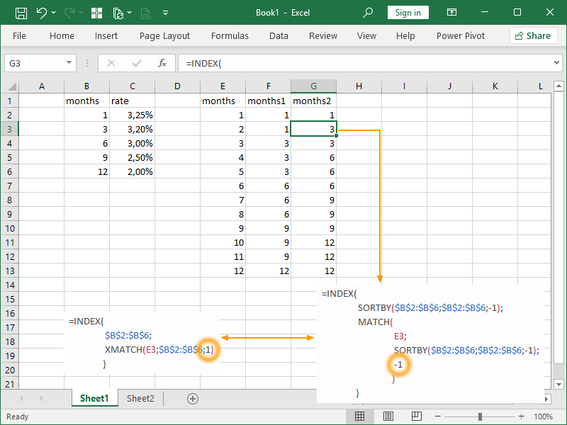
We can use the match type -1 (greater than or equal to) in order to retrieve the first larger value than the one we are looking up.
As our lookup array ($B$2:$B$6) is sorted from smallest to largest, we will have to sort it from largest to smallest first.
In this example, we will use the SORTBY function in order to sort our lookup array and our return array from largest to smallest. Both arrays have to be sorted in the same way:
With the XMATCH function, we are using match type -1 (exact match or next smaller item).
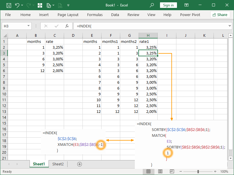
We can use match type 1 (less than or equal to) in order to retrieve the first rate related to a smaller period than the one we are looking up.
Our lookup array ($B$2:$B$6) is already sorted from smallest to largest, so no additional sorting is needed.
However, that may not always be the case. In the following example, we will also use the SORTBY function in order to sort our lookup array and our return array. Both arrays have to be sorted by the same sorting array:
With the XMATCH function, we are using match type 1 (exact match or next smaller item).
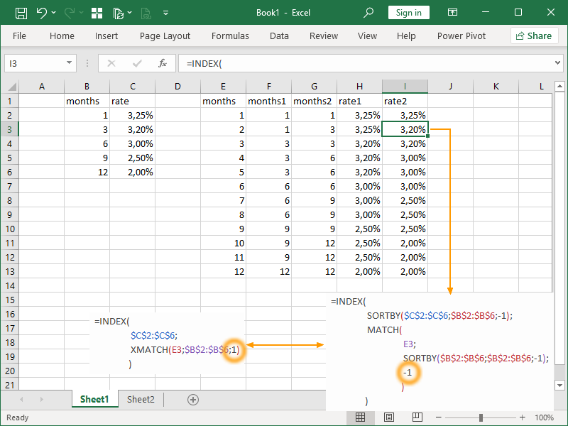
We can use the match type -1 (greater than or equal to) in order to retrieve the first rate related to a larger period than the one we are looking up.
As our lookup array ($B$2:$B$6) is sorted from smallest to largest, we will have to sort it from largest to smallest first.
In this example, we will use the SORTBY function in order to sort our lookup array and our return array. Both arrays have to be sorted in the same way and by the same sorting array:
With the XMATCH function, we are using match type -1 (exact match or next smaller item).
Once we’ve returned all the necessary periods and rates, we can use the FORECAST.LINEAR function in order to interpolate the missing rates:
Now consider the following example.
We have a list of exchange rates for several different dates and currencies.
That list has no available dates for weekends. We need to retrieve an exchange rate for a specific Saturday, so we want to use the exchange rate for the previous day, Friday.
The list is already sorted in ascending order (oldest to newest date), and we are using structured references:
By using match type 1 (less than or equal to), we’ve retrieved the first smaller value available on the list, i.e., the EUR USD exchange rate for the previous day.
This is probably not what we want. We also want to specify the currency code available in the column code.
However, we can’t look up multiple criteria here, as this is only possible with match type 0 (exact match).
In order to retrieve the first smaller exchange rate available on the list for, let’s say, the GBP currency code, we will have to first filter that list:
By using the FILTER function, we can generate an array that will contain only exchange rates for the GBP currency code and then retrieve the exchange rate for the previous day, Friday.
Logic of the less than or equal to and greater than or equal to matching demonstrated here also applies to the XLOOKUP function, but with differences in syntax and requirements. See this article on how to use the XLOOKUP function for this purpose.
Dig deeper:
Lookup with unique identifiers
Lookup the 2nd, the 3rd, or the nth value


2 thoughts on “How to use less than or greater than MATCH”