UNIQUE function

The UNIQUE function replicates and extends Excel’s Remove Duplicates feature in formula form.

The UNIQUE function allows us to return a list of unique values in a list or range.

By default, the UNIQUE function will return multiple values, which will be placed in the neighboring cells (to the bottom and/or to the right). I.e., we are dealing with dynamic array formulas here.

 

The syntax of the UNIQUE function is as follows:

= UNIQUE ( array ; [by_col] ; [exactly_once] )

The (return) array represents an array or a range of cells to return values from.

The by_col logical value (TRUE or FALSE) can be used to change the comparison direction. If omitted, it defaults to FALSE (duplicate rows are removed).

The exactly_once logical value (TRUE or FALSE) can be used to return only items that occur only once. If omitted, it defaults to FALSE (every distinct item is returned).

 

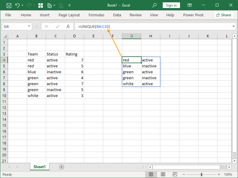
We can retrieve unique values (remove duplicate values) from a single column in the following way:

 

We can retrieve unique combinations of values (remove duplicate combinations of values) from two or more columns in the following way:

 

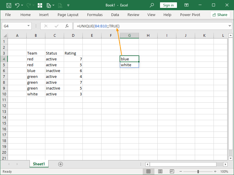
We can retrieve values that occur once in the following way:

If we try this with multiple columns, we will retrieve unique combinations of values that occur once.

 

We can combine the UNIQUE function with the SORT function in order to generate a sorted list of unique values:

Note, when combining UNIQUE and SORT functions, it is irrelevant which one is nested in the other. It is the same if we sort our values and then remove duplicates, or if we remove duplicates and then sort that list.

 

We can combine the UNIQUE function with the FILTER function in order to generate a list of unique values that meet certain criteria:

In this example, we have two rows that contain red, active, and a rating equal to or higher than 5. Both meet the filtering criteria, and a duplicate one is removed with the UNIQUE function.

We also have no rows that contain white, active, and a rating equal to or higher than 5. The FILTER function will not return that row, and it will not be taken into consideration by the UNIQUE function.

 

We can also combine the UNIQUE function with both the SORT function and the FILTER function in order to generate a sorted list of unique values that meet certain criteria:

The return of this combination of functions is the same as in the previous example, only sorted.

 

We can nest any array in the UNIQUE function in the same way we’ve nested the returns of the SORT and FILTER functions.

Formulas such as the one where the XLOOKUP function is nested

=UNIQUE(XLOOKUP(“Team”;B3:C3;B4:C10))

or an array of concatenated values is nested

=UNIQUE(B4:B10&” “&C4:C10)

are perfectly legitimate.

 

One final note: both workbooks have to be open if you are returning a list of unique values from a different workbook.

 

Dig deeper:

Remove Duplicates feature

Sort & Filter in Excel

FILTER function