
When analyzing large amounts of data in Excel, often the best approach is to retrieve the top (10) values.
Consider the following example:

This table contains all of the invoices from January 29th. There are 904 invoices for that day.
The values in the invoice column are unique, as those are invoice numbers.
The values in the user column are not unique, as some users have multiple invoices on that day, and the values in the team column are not unique, as there are only five teams.
The values in the EUR amount column are also not unique, as amounts charged are also repeating— there are many invoices of the same amount.
We are obviously interested in our top invoices. With the help of the LARGE, COUNTIFS, and SUMIFS functions, we can easily retrieve some information about the list we need to generate:

The 10th largest invoice amounts to EUR 97,99. However, there are 11 invoices amounting to EUR 97,99 or more, as our 11th largest invoice is of the same amount as our 10th largest invoice. The sum of those 11 largest invoices is EUR 1.084,89.
Top 10 lists in Excel with Sort & Filter
Filtering is often used in order to retrieve the top 10 values. We will use Sort & Filter in our examples here, but the same principles and limitations apply to Excel Tables.
For example, we can sort our EUR amount column by size in order to retrieve the largest invoices:
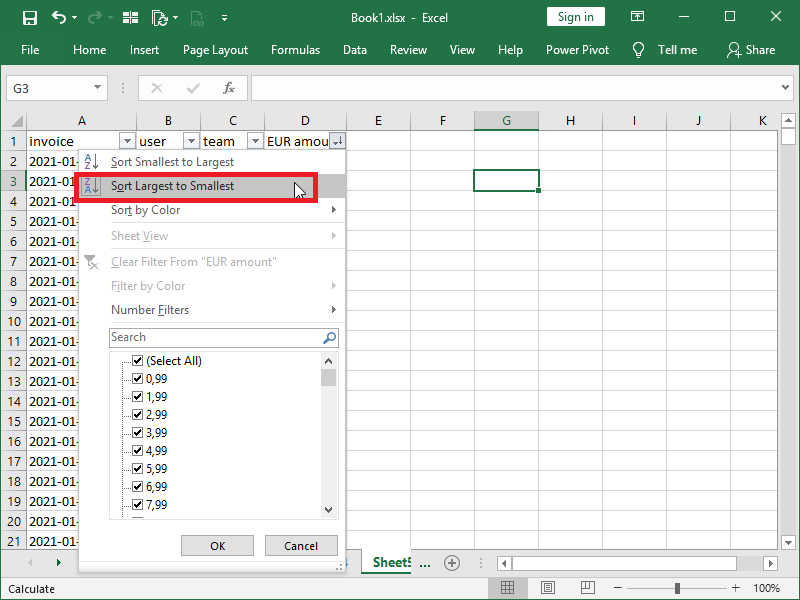
This is what our “top 10” list looks like:

Excel AutoFilter also contains a built-in Top 10 feature, which is able to select top or bottom, 10 or some other number, items, or percent of items:

This is how our data would look if we had applied the Top 10 filter (top 10 items) to column D and then additionally sorted our data from largest to smallest:

However, this is simple only because invoice numbers are unique.
Generating the top 10 billed users’ list is more complicated. Our first order of business would be to copy our user list into a new column and remove duplicates:
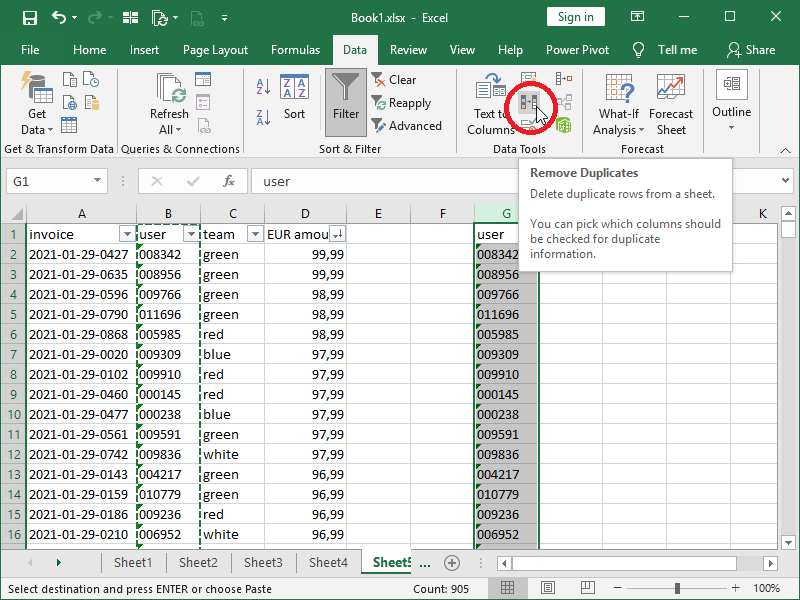
Next, we would have to use the SUMIFS function in order to retrieve amounts billed to users and then sort those values by size in order to generate a list of the top-billed users:

Top 10 lists in Excel with Pivot Tables
Ideal tool for this kind of analysis in Excel are Pivot Tables, a technique of arranging and rearranging data in order to draw attention to useful information.
We start by selecting our data and creating a new pivot table:
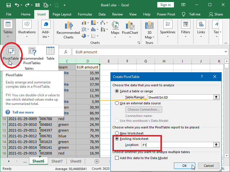
As we are interested in top invoices, we drag the invoice filed to Rows, and we drag the EUR amount to Values. There are multiple options available on how to show values here, but for our purposes, Sum of EUR amount, the default one, is suitable:

Next, we sort our Row Labels in descending order by the Sum of EUR amount:
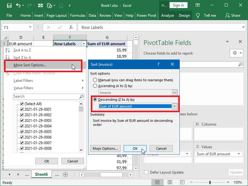
Then, we filter our Row Labels with the Top 10 filter by the Sum of EUR amount:
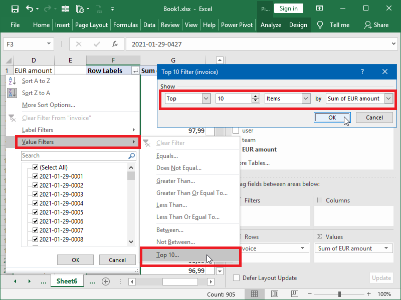
This is our result:
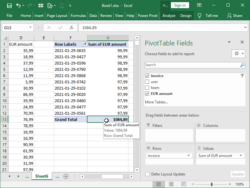
Note that this list by default contains 11 invoices, as the 11th largest invoice is for the same amount as the 10th largest invoice.
Note also that our invoice numbers are not sorted and can’t be sorted by invoice number.
Using the same principles, it is also easy to generate our Top 10 users list:

Pivot Tables also enable us to quickly do more.
For example, if we want to include invoices in our users list, we can show invoices billed to our top users by dragging the invoice filed under the user field in the Rows area:

This can also be further expanded, with pivot tables offering a wide range of possibilities, such as filtering the top 10% of items, filtering items greater, equal, or smaller than a certain amount, counting, averaging, and more.
Top 10 lists in Excel with legacy array formulas
Some combination of INDEX and MATCH functions, SUMIFS and COUNTIFS functions, LARGE and SMALL functions, ROW and ROWS functions, RANK functions, and INDIRECT function is typically used to generate the top 10 list with formulas, as are conditional statements.
Note, formulas applied here could lead to performance issues when used on large datasets.
If list items are unique in the original dataset, we can retrieve the top 10 list with these formulas:
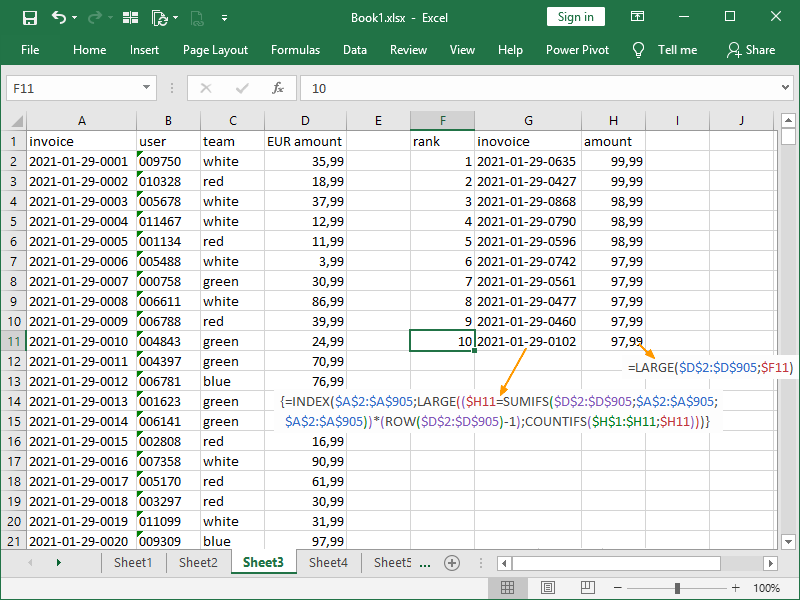
Our formulas are:
=LARGE($D$2:$D$905;$F11)
{=INDEX($A$2:$A$905;LARGE(($H11=SUMIFS($D$2:$D$905;$A$2:$A$905;$A$2:$A$905))*(ROW($D$2:$D$905)-1);COUNTIFS($H$1:$H11;$H11)))}
What is going on here?
In column H, we are retrieving the largest values. We can do this in this simple way, using only the LARGE function, because invoice numbers are unique.
As EUR amounts are not unique, we cannot just match our amounts with corresponding invoice numbers; in column G, we will have to use array formulas.
First, we will have to check all of the possible rows where our sum amount appears.
Those FALSE or TRUE results are multiplied by an index of row numbers generated by the ROW function; for FALSE results, zeros will be returned, and for TRUE results, positions in an index will be returned.
As we have several of those positions, we will retrieve one of them with the help of the LARGE function. Here, we are retrieving the count of until this row appearing invoice values the largest value, and our last appearing invoices of the same value will be shown first. The opposite sorting can be achieved by applying the SMALL function.
In the final step, we are retrieving the invoice number located in the position specified by the LARGE function.
Note that, as we didn’t specifically look up the amount of our 11th invoice (12th, 13th, etc.), we’ve added only ten invoices to the list. Had we applied different sorting, one different invoice would be present on our list.
If list items are not unique in the original dataset, we can retrieve the top 10 list with these formulas:
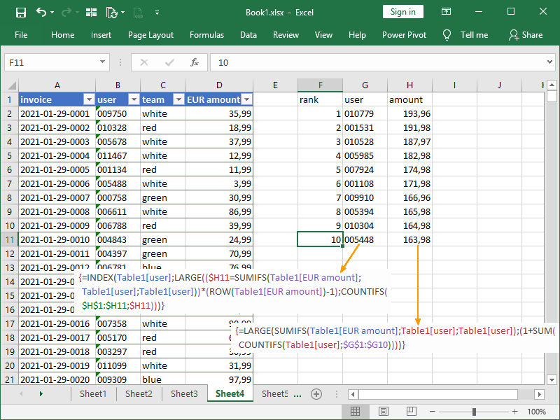
Our formulas are:
{=LARGE(SUMIFS(Table1[EUR amount];Table1[user];Table1[user]);(1+SUM(COUNTIFS(Table1[user];$G$1:$G10))))}
{=INDEX(Table1[user];LARGE(($H11=SUMIFS(Table1[EUR amount];Table1[user];Table1[user]))*(ROW(Table1[EUR amount])-1);COUNTIFS($H$1:$H11;$H11)))}
What is going on here?
Aside from the fact that we’ve formatted our data as an Excel Table and are using structured references for simplicity, further complications have arisen.
As our list members (users) are no longer unique, we now have to use an array formula to retrieve the largest amounts.
We had to create an array that contains the sum of the EUR amount per user in all rows. With the help of the LARGE function, we will next retrieve the largest value (n, the number of appearances of user numbers from previous ranks in our complete data set).
Once we’ve successfully accomplished that task, we can retrieve user names using the same principles as in our previous example.
Note that not only is our column G again referencing column H, but column H is now also referencing column G.
Top 10 lists in Excel with dynamic array formulas
In Office 365 (Microsoft 365) and Microsoft Office 2021 and later, some combination of the FILTER function, SORT and SORTBY functions, UNIQUE function, and SEQUENCE function can be used to generate the top 10 lists with formulas.
Those can be combined in multiple ways, and we will show two relatively simple examples here.
If list items are unique in the original dataset, we can retrieve the top 10 lists with these formulas:
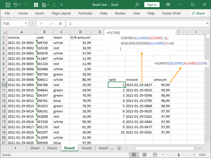
Our formulas are:
=FILTER(SORTBY(A2:A905;D2:D905;-1);SEQUENCE(ROWS(A2:A905))<=10)
=SUMIFS(D2:D905;A2:A905;G10#)
What is going on here?
In column G, we are combining FILTER with SORTBY and SEQUENCE functions in order to retrieve the top 10 invoices (invoice numbers are unique).
First, we’ve used the SORTBY function to select invoice numbers and sort them in descending order based on invoice amounts.
Next, we’ve nested the return of the SORTBY function into the FILTER function, where we’ve filtered in only the first 10 items from that sorted list (by applying filtering criteria to a corresponding array generated by the SEQUENCE function).
In column H, we’ve retrieved the corresponding values for those invoice numbers using the SUMIFS function.
If list items are not unique in the original dataset, we can retrieve the top 10 lists with these formulas:
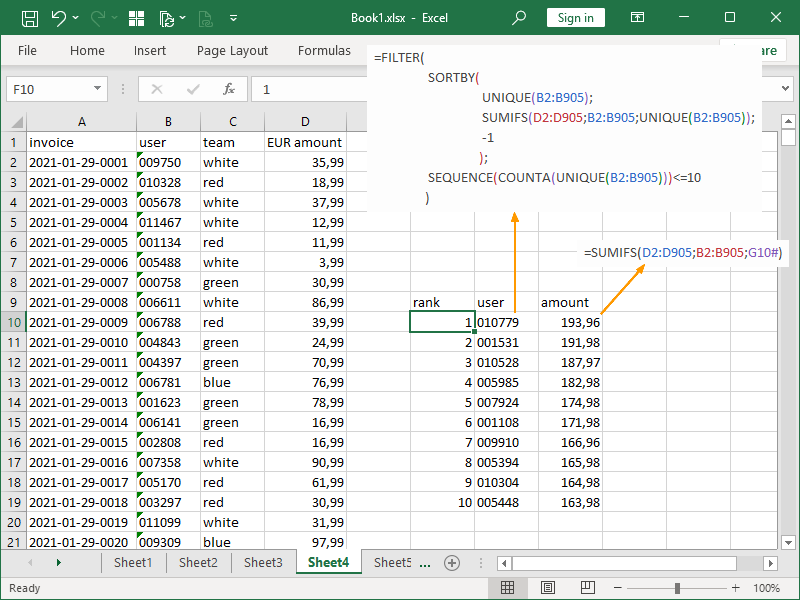
Our formulas are:
=FILTER(SORTBY(UNIQUE(B2:B905);SUMIFS(D2:D905;B2:B905;UNIQUE(B2:B905));-1);SEQUENCE(COUNTA(UNIQUE(B2:B905)))<=10)
=SUMIFS(D2:D905;B2:B905;G10#)
What is going on here?
In column G, we are combining FILTER with SORTBY, UNIQUE, SUMIFS, and SEQUENCE functions in order to retrieve the top 10 users (user codes are not unique; there are sometimes multiple invoices per user).
First, we’ve used the UNIQUE function to generate a list of unique user codes. We’ve also created an array of SUMIFS function returns where sums are generated for a list of unique user codes.
Next, we’ve used the SORTBY function to sort our list of unique user codes in descending order, based on the corresponding array of sums for that same list of unique user codes.
Next, we’ve nested the return of the SORTBY function into the FILTER function, where we’ve filtered in only the first 10 items from that sorted list (by applying filtering criteria to a corresponding array generated by the SEQUENCE function).
In column H, we’ve retrieved the corresponding sums for those user codes using the SUMIFS function.
Dig deeper:
3 thoughts on “Top 10 lists in Excel”