Combining INDIRECT with ADDRESS

We’ve previously covered how we can use any function to generate a text that could be a valid cell reference, both the column and row parts of the address, and then use the INDIRECT function to convert that text to a cell reference. This process can be greatly enhanced by the ADDRESS function.

 

The ADDRESS function returns a text string that represents the address of a particular cell.

Row, column, type of reference (locked or absolute), reference style (A1 or R1C1 style), and worksheet can be specified in the arguments.

 

The ADDRESS function syntax is as follows:

= ADDRESS ( row_num ; column_num ; reference_type ; reference_style ; “[workboook]worksheet” )

Row number is a numeric value that specifies the row to be used in the cell reference.

Column number is a numeric value that specifies the column to be used in the cell reference.

Reference type is a numeric value that specifies the type of reference to be used in the cell reference, with 1 representing absolute references. If omitted, absolute references will also be used.

Reference style is a numeric value that specifies the style of reference to be used in the cell reference, with 1 representing A1 reference style. If omitted, A1 reference style will also be used.

Worksheet and potentially workbook parts of the address are entered in the final argument, inside quotation marks, as text. Valid examples are “Sheet1” or “[Book1]Sheet1”. You will, however, not be able to reference closed workbooks in this way. If omitted, the current worksheet will be referenced.

 

Consider the following example:

In column E, we have generated a number of text strings that represent cell addresses, both inside and outside the current worksheet / workbook.

We are always first specifying a row, then a column, then a reference type, then a reference style, and at the end, a worksheet and eventually a workbook:

 

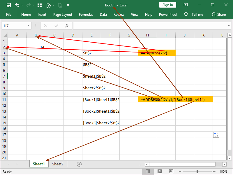
Given that those are valid references, we can put our returns as arguments for the INDIRECT function and return the figures in referenced cells:

Note the #REF! error in the H15 cell – as Book3 is currently closed, that reference is hence not valid!

 

We can combine those functions directly by nesting the ADDRESS function inside the INDIRECT function, as shown in cell H17:

 

We can also combine two ADDRESS functions in a text string in order to generate a reference to a cell range. Once generated, that text string can be nested inside the INDIRECT function, and operations performed with it:

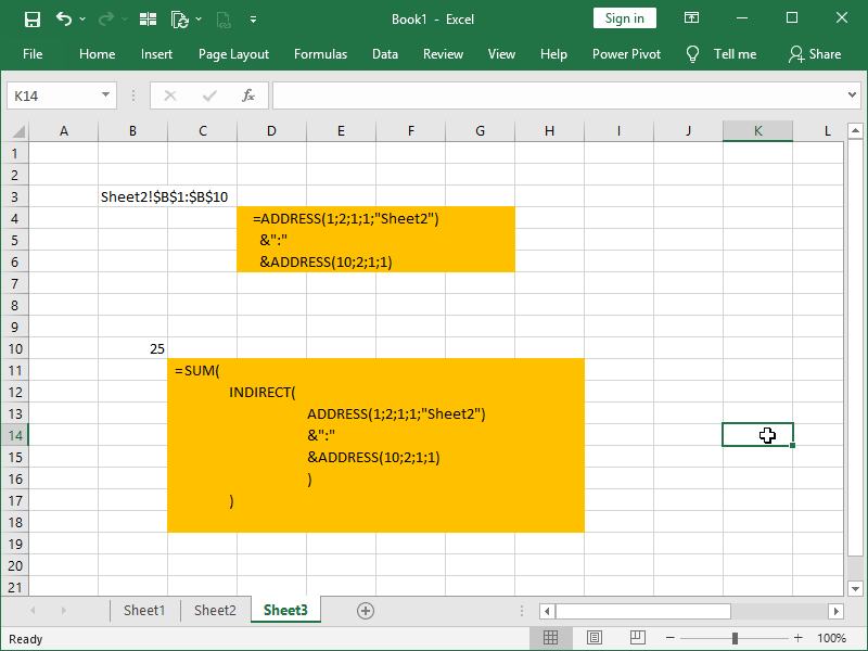
Note that when calculating the final cell in the range (second ADDRESS function), we are not referencing the worksheet.

 

Now consider this practical example:

Every month, we are receiving YTD data in this structure, i.e., every month, a new column and possibly several rows are added if new users and teams appear.

What is our last YTD?

What is our last MTD?

What is our last YTD for a particular user?

What is our last MTD for a particular team?

Answers to such questions can easily be automated and momentarily available with the help of the INDIRECT ADDRESS returns combined with other needed functions:

Assuming the same data structure, by counting filled rows and columns, we can generate indirect references to the last periods. Once set up, these kinds of, admittedly complex, formulas can provide us with the required answers indefinitely. In every future period, our only additional work would be to paste new export to the “data” sheet.

There are, naturally, other ways to achieve these results, but situationally, the INDIRECT ADDRESS combination will be the simplest or even the most robust solution.

 

Dig deeper:

INDIRECT function

How to use the INDIRECT function to define function arrays

Text in Excel