Two related sorting functions, SORT and SORTBY, replicate and extend Excel AutoFilter sorting functionality in formula form.
The SORT function can be used to sort the contents of a range or array based on the values in that range or array, while the SORTBY function can be used to sort the contents of a range or array based on the values in the corresponding range or array, as illustrated here:
By default, these functions will return multiple values, which will be placed in the neighboring cells (to the bottom and/or to the right). I.e., we are dealing with dynamic array formulas here.
The SORT function sorts the contents of a range or array based on the values in that range or array.
The syntax of the SORT function is as follows:
= SORT ( array ; [sort_index] ; [sort_order] ; [by_col] )
The (return) array represents an array or a range of cells to sort.
The sort index number specifies a column to sort by. If omitted, it defaults to 1; the array will be sorted by the first column.
The sort order number specifies the order of sorting: 1 for ascending order (smallest to largest) and -1 for descending order (largest to smallest). If omitted, it defaults to 1 (smallest to largest).
The by_col logical value (TRUE or FALSE) can be used to change the sorting direction. If omitted, it defaults to FALSE (rows in columns are sorted).
We can select a single column from a cell range and sort it in the following way:
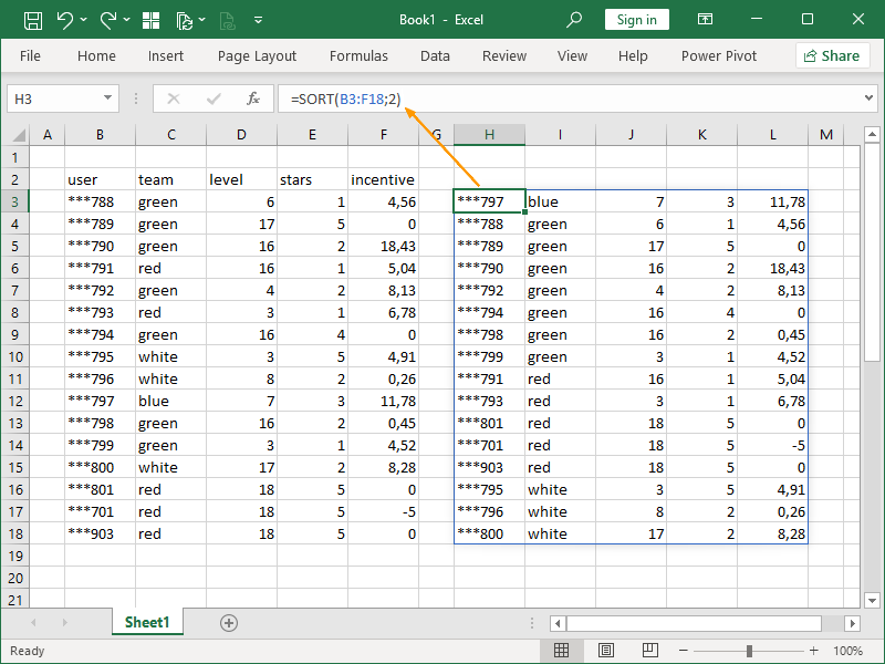
We can select multiple columns from a cell range and sort them in the following way:
We are again sorting by the cell range C3:C18.
However, in order to do that, as we are now sorting the whole range, we have to specify our sort index number as 2 (2nd column in the selected cell range).
Had we not done so, our formula would default to sorting by the cell range B3:B18.
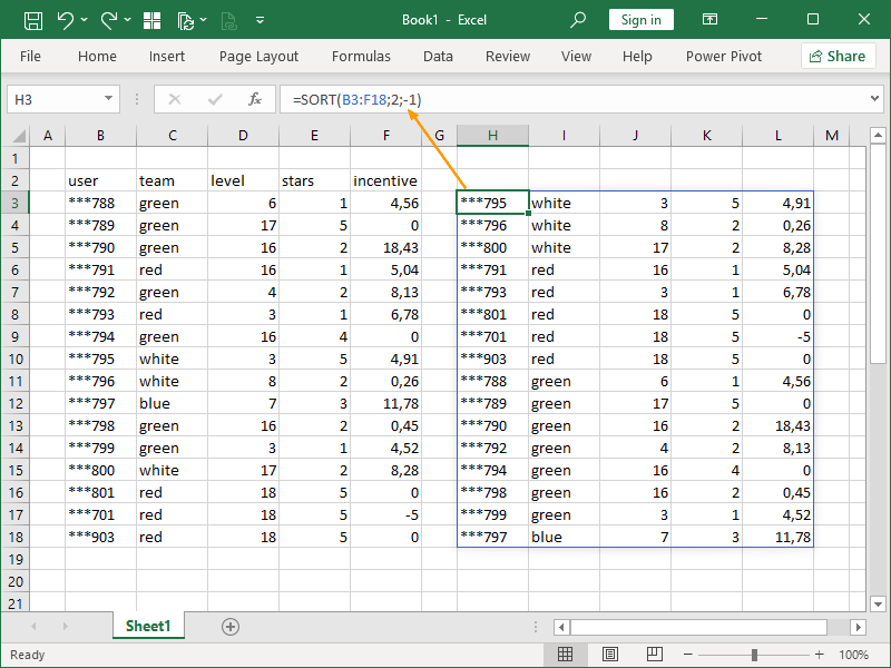
We can sort in the descending order (largest to smallest) by specifying the sort order as -1:
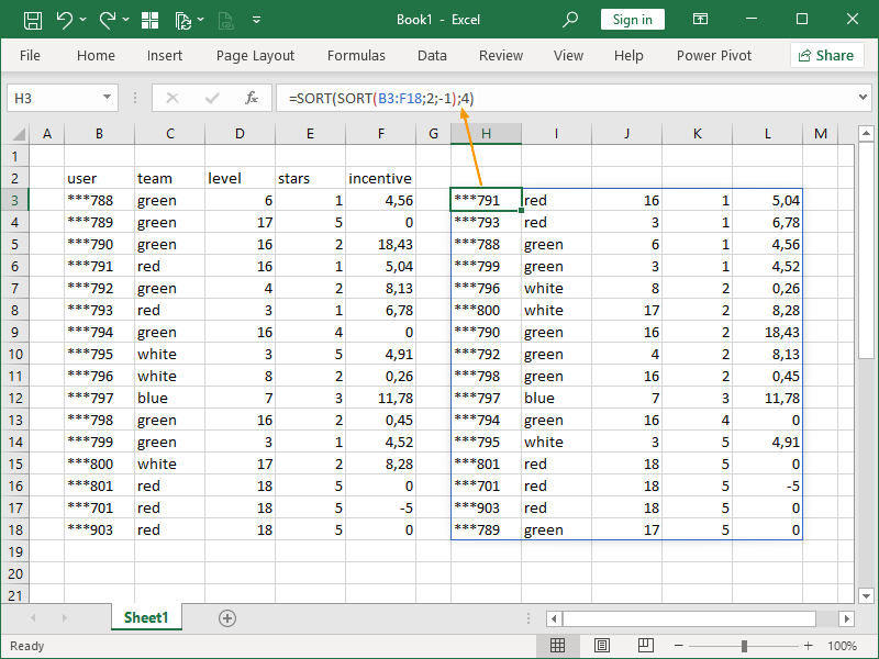
The simplest way of sorting by multiple columns can be accomplished by combining multiple SORT functions:
In this particular example, we’ve sorted the cell range B3:F18 by the cell range C3:C18, ordered descending, and then sorted that result by the 4th column in the return array, which is the same as sorting by the cell range E3:E18.
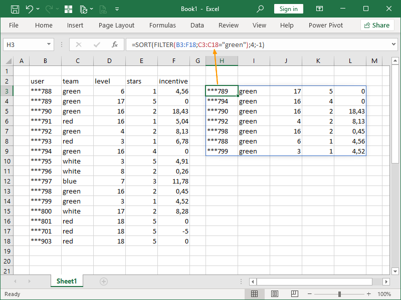
We can also combine the SORT function with the FILTER function in order to sort filtered values:
In this example, we’ve filtered the rows where values in the cell range C3:C18 are equal to green and then sorted that array by the fourth column in descending order.
The SORTBY function sorts the contents of a range or array based on the values in the corresponding range or array.
The syntax of the SORTBY function is as follows:
= SORT ( array ; by_array_1 ; [sort_order1] ; … )
The (return) array represents an array or a range of cells to sort.
Multiple corresponding arrays to sort by can be defined, but only one has to be defined.
The sort order number specifies the order of sorting: 1 for ascending order (smallest to largest) and -1 for descending order (largest to smallest). If omitted, it defaults to 1 (smallest to largest).
With the SORTBY function, the sorting direction is defined by the characteristics of the corresponding array to sort by.
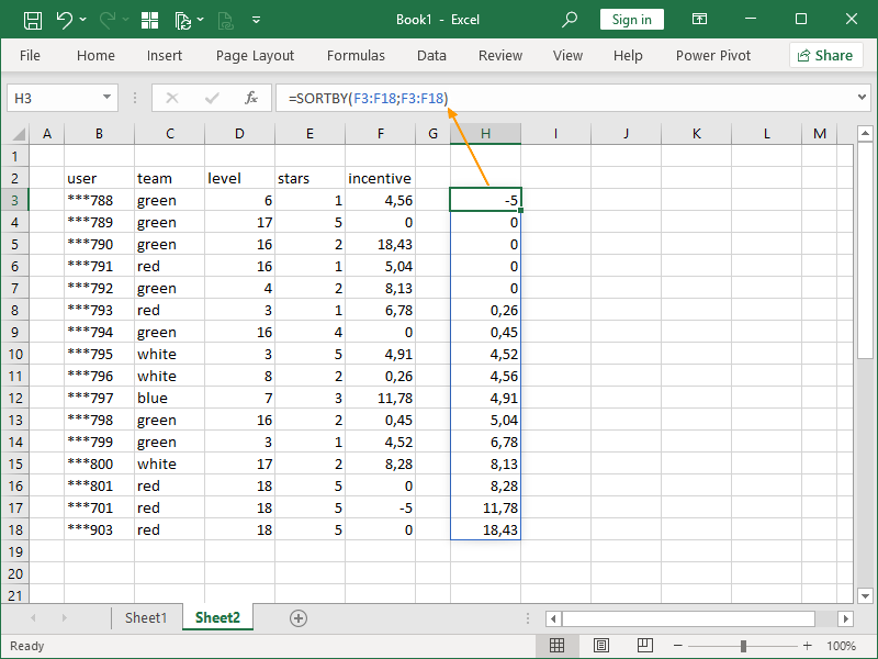
We can select a single column from a cell range and sort it in the following way:
Note the different approach compared to the SORT function.
Here, we have to enter the cell range we want to sort twice.
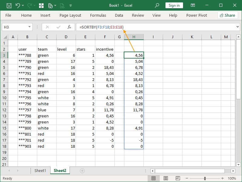
We can select a single column from a cell range and sort it by a different column in the following way:
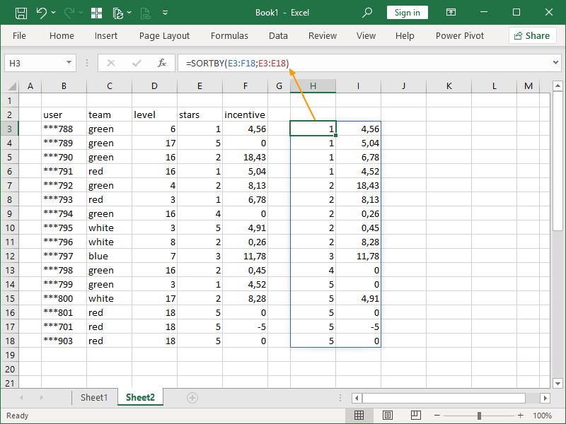
We can also select multiple columns from a cell range and sort it by any given column in the following way:
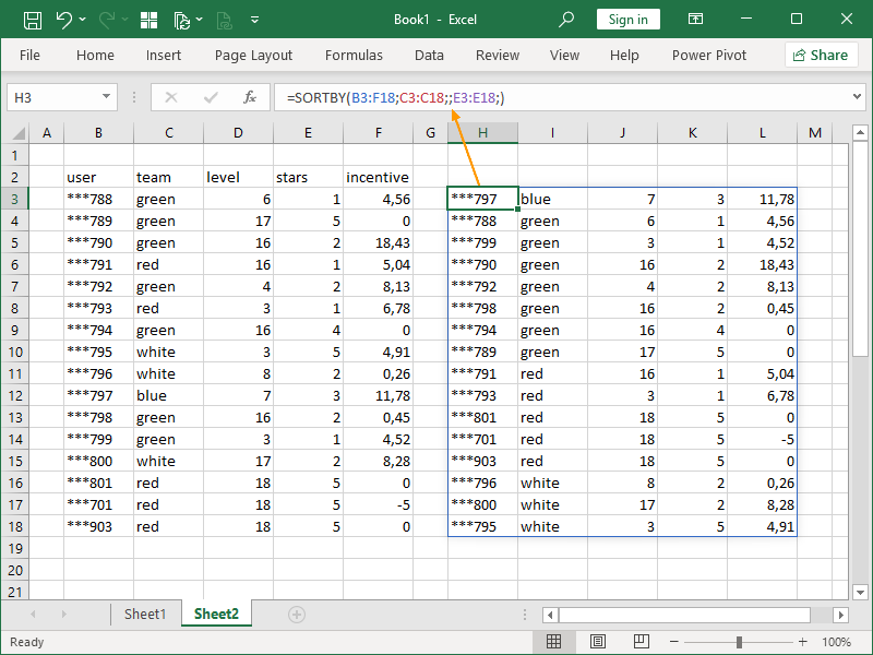
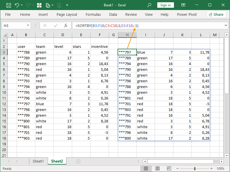
We can also select multiple columns from a cell range and sort it by any given multiple columns in the following way:
In this example, we’ve sorted the cell range B3:F18 by the cell range E3:E18, and then sorted that result by the cell range C3:C18.
Or at least, that would be the procedure had we used Excel’s AutoFilter sorting functionality.
In the SORTBY function, we’ve just designated the cell range C3:C18 as our first sort by array and the range E3:E18 as our second sort by array.
We can also sort in descending order (largest to smallest) by specifying the sort order as -1:
This example is the same as the previous one on the first sorting level (team), given that the omitted sorting order number defaults to 1 (smallest to largest).
However, on the second sorting level (stars), our values are sorted from largest to smallest now, given that we’ve specified descending sorting order with the -1 in the sort_order2 part of the argument.
In our examples so far, we’ve always used columns from the tables we were sorting as our corresponding arrays. However, one of the great strengths of the SORTBY function is that we didn’t have to; we could have used any array of the appropriate size.
We can build custom sort by arrays for the SORTBY function and, with them, perform various types of custom data sorting.
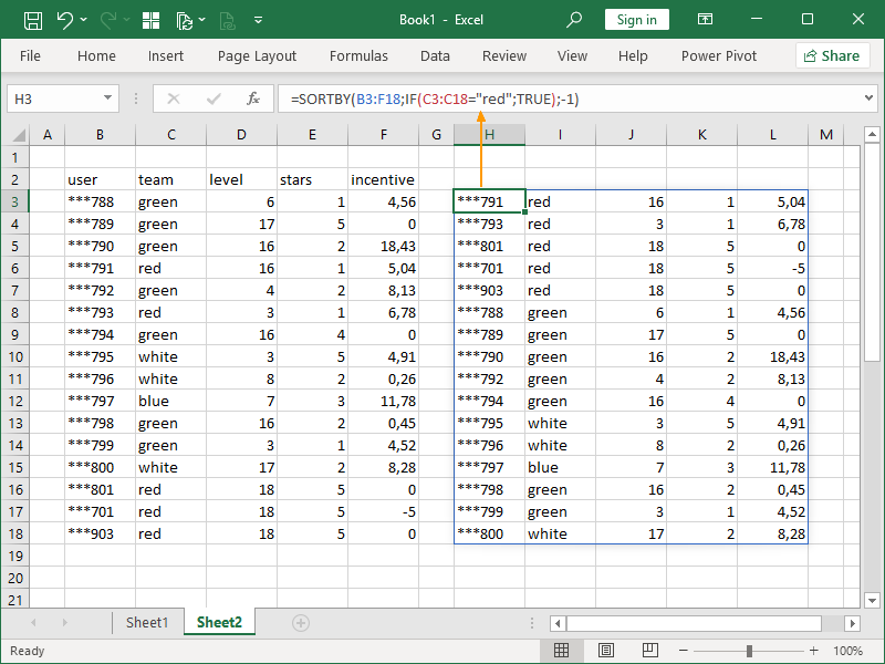
We can combine the SORTBY function with the IF function in order to sort data based on whether certain criteria are met.
Consider the following example:
Here, we’ve sorted our table based on whether the team in the cell range C3:C18 equals red. If the team equals red, those rows are returned first, and all other rows follow.
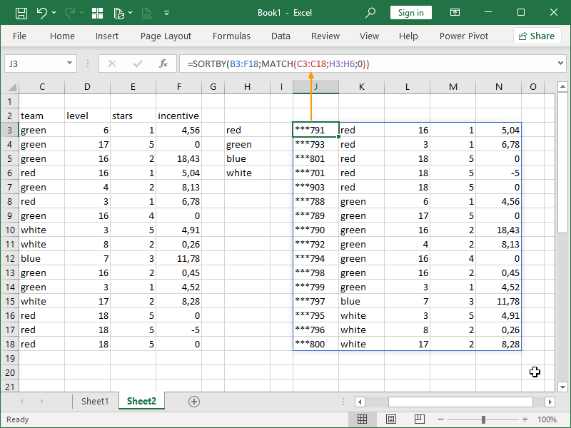
We can combine the SORTBY function with the MATCH function in order to sort data based on a custom list we’ve built.
Consider the following example:
Here, we’ve sorted our table according to the mapping in the cell range H3:H6.
If needed, we can change our mapping in the cell range H3:H6, and our SORTBY return would also automatically change.
One final note: both workbooks have to be open if you are sorting from a different workbook.
Dig deeper:


4 thoughts on “SORT & SORTBY functions”