We’ve previously established the rules for writing criteria in the SUMIFS function:
- we can reference any cell
- we can enter any number directly into the function
- we can enter text directly in the function, nested inside quotation marks “”
- a logical test is nested inside of quotation marks “”, with the comparison operator coming first and a number second.
We will further expand on the topic in this article.
Formulas and functions can also be nested in SUMIFS criteria.
If needed, both can be combined with logical tests.
We can nest formulas in the SUMIFS function criteria by enclosing them in parenthesis ().
Consider the following example:
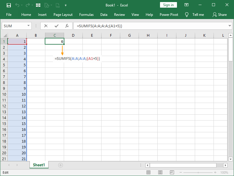
We have a list of numbers from 1 to 100, and we want to sum the numbers that are equal to 6. Instead of just writing 6 in the criteria, we can also nest a formula between parenthesis. The SUMIFS function is returning the sum of all the numbers in column A equal to 6 – just one in this example.
Another thing we can do is nest functions in the criteria:
In this example, the SUMIFS function is returning the sum of all the numbers in column A equal to the smallest number, 1.
These principles become obviously useful when combined with conditional statements.
A logical test is usually nested inside quotation marks “”, with the comparison operator coming first and a number (or text) second. However, this will not work with formulas and functions, as they will be treated as text and not calculated.
In order to combine logical tests with formulas and functions, we first have to nest the logical operator inside of quotation marks “”, use an ampersand &, and only then write our function or formula.
All of the available Comparison operators can be used:
equal to =
greater than >
greater than or equal to >=
less than <
less than or equal to <=
not equal to <>
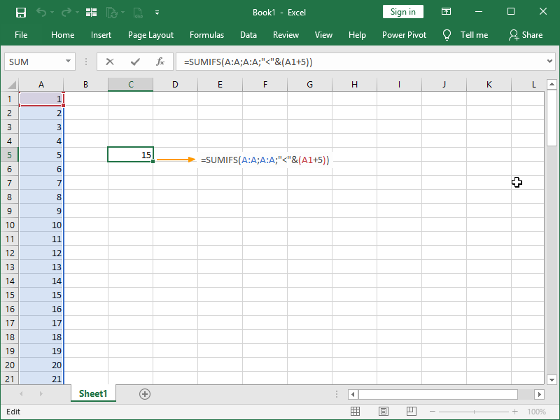
We could write a formula that will sum only numbers smaller than 6 in this way:
We would return 15, as that is the sum of numbers smaller than 6, cells A1 to A5.
We could write a formula that will sum only numbers smaller than average in this way:
We would return 1275, as our average is 50,5 and, with the given criteria, our formula will only sum the numbers smaller than that number, cells A1 to A50, returning 1275.
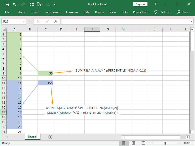
What if we want to only sum the numbers below the 10th percentile, i.e., 10% of the lowest values?
We would use this formula:
=SUMIFS(A:A;A:A;”<“&PERCENTILE.INC(A:A;0,1))
What if we want to only sum the numbers between the 10th percentile and the 20th percentile?
We could sum the values below the 20th percentile and subtract the sum of the values below the 10th percentile, like this:
=SUMIFS(A:A;A:A;”<“&PERCENTILE.INC(A:A;0,2))-SUMIFS(A:A;A:A;”<“&PERCENTILE.INC(A:A;0,1))
This is what the returns would look like:
Dig deeper:


3 thoughts on “SUMIFS criteria: formulas, functions and conditional statements”