Lookup with unique identifiers

INDEX function

The INDEX function returns the value from a range of cells based on the row and column specified in the function arguments.

We are simplifying here: the INDEX function can actually return values from one or more arrays, i.e., a broader term for lists of data that includes cell ranges. But the most common use is with cell ranges, as that is the typical way of structuring data in Excel.

 

The syntax of the INDEX function is as follows:

= INDEX ( array ; row_num ; column_num )

Array will, in our case, always be defined as a range of cells, such as C6:G10 – think of it as a new “virtual” table that is created inside of the INDEX function based on values from a range of cells, such as C6:G10.

The row number is always an integer, such as 0, 1, 2, 3,…

A column number is always an integer, such as 0, 1, 2, 3,…

 

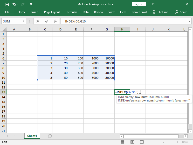
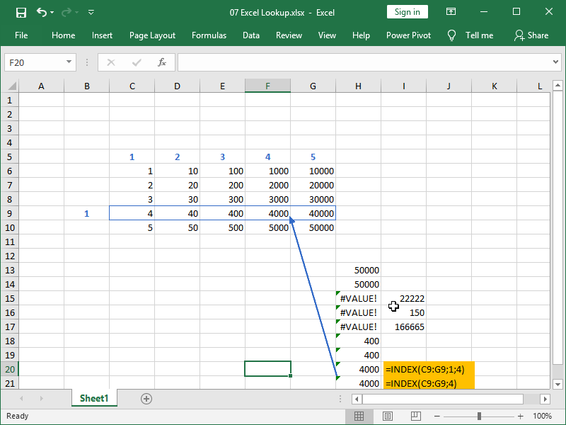
Here is what the basic application of the INDEX function looks like:

Here, we created our new “virtual” table from the data in cell range C6:G10.

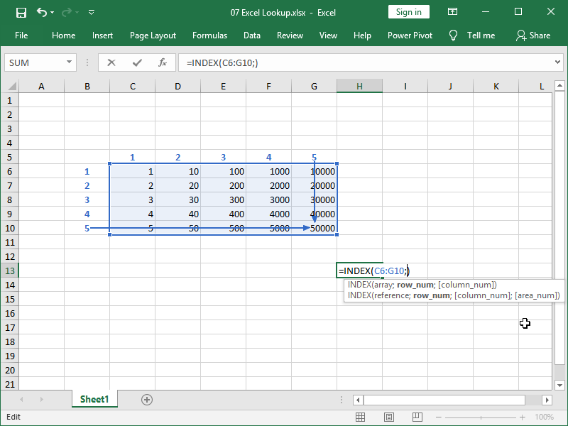
In the INDEX function, the number 50000 is not in cell G10 but rather inside of a “virtual” table existing only in our INDEX function, with an address in row 5 and column 5:

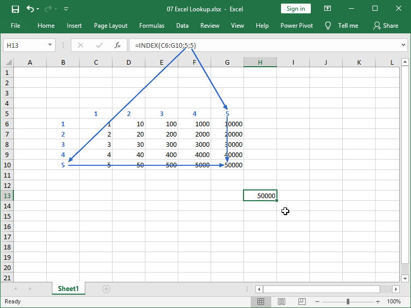
Indeed, if we set the row number to 5 and the column number to 5, our function will return the number 50.000:

 

It doesn’t matter how we set or calculate those row and column integer numbers (and if we input decimal numbers, they will be rounded down to integer numbers anyway).

We can do it in the most nonsense-like ways, such as by referring to the cells that we included in our “virtual” table:

 

If we want to return the whole row, we can do that by defining the desired row and then defining the column as zero.

If we want to return the whole column, we can do that by defining the desired column and, before that, defining the row as zero.

If we want to return the whole table, we can do that by defining both column and row as zero.

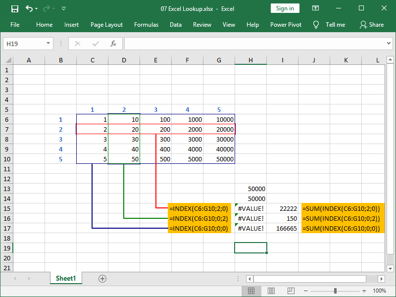
Returning the whole array of numbers into a single cell is not really what you can realistically do in Excel, but you can, for example, sum that array of numbers:

Here, we are returning row number 2, column number 2, or the whole table with the help of the INDEX function, which results in errors.

However, if we nest the INDEX function inside the SUM function, instead of errors, we will return the sum of the desired row, column, and table, respectively.

 

It is often the case that your array will consist of only one column, such as E6:E10 in the example below.

In the column number part of the argument, valid statements are then either zero or number 1, as shown in cell H19.

You can also omit column number part or the argument, which the INDEX function will interpret as if you’ve entered number 1:

The same is true for arrays consisting of only one row. However, omitting the row number part of the argument is not exactly a good practice in writing INDEX formulas and can lead to issues down the line.

 

MATCH function

The MATCH function returns the relative position of the item in the range, either a row or a column.

The relative position is returned in the form of an integer number, such as 1, 2, 3,…

 

The syntax of the MATCH function is as follows:

= MATCH ( lookup_value; lookup_array; match_type)

The lookup value can be either a text or a number, inputted directly into the function or as a cell reference.

The lookup array will, in our case, always be defined as a range of cells, such as C3:C7. Again, think of it as a new “virtual” table that is created inside of the MATCH function based on values from a range of cells, such as C3:C7.

The difference here is that we are dealing with either a row or a column. An integer number returned is always the relative position of our lookup value in the range.

The match type should always be zero 0, i.e., we will be looking for exact matches.

 

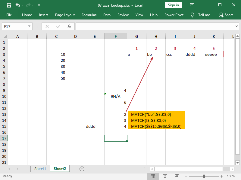
This is what the basic application of the MATCH function looks like:

In cell F9, we are retrieving the relative position of number 40 inside an array C3:C7, and that relative position is represented by an integer number 4.

In cell F10, we are doing the same for the text “40”, but as our array C3:C7 doesn’t contain such text, an error is returned.

 

Be careful when designating your arrays; blank cells are counted:

 

Next, this is an example of the MATCH function applied to data in a row:

In cell F13, we are retrieving the relative position of the text “bb” from an array C3:C7, and that relative position is represented by an integer number 2.
In cells F12 and F13, we are doing the same for other text strings, but we are also referencing them from cells.

 

The MATCH function is not case-sensitive and can perform matches with text strings up to 255 characters long.

Partial matches with the help of an asterisk * or a question mark ? are also supported, as long as the match type is defined as zero. A formula such as =MATCH(“cc?”;G3:K3;0) will return number 3 in our example.

Match type, other than 0, exact match, can be:

• 1, less than, finds the largest value that is less than or equal to the lookup value, while the lookup array must be placed in ascending order,
• -1, greater than, finds the smallest value that is greater than or equal to the lookup value, while the lookup array must be placed in descending order.

For more details, see this article on how to use the less than or greater than match type.

Both partial matches and non-exact matches, while useful in the right context, are to be avoided if we want to look up data with unique identifiers.

 

How to combine INDEX with MATCH

We can use the INDEX function to designate a cell range from which we want to retrieve data and, at the same time, use the MATCH function to specify the address of a cell in that range, i.e., row and column.

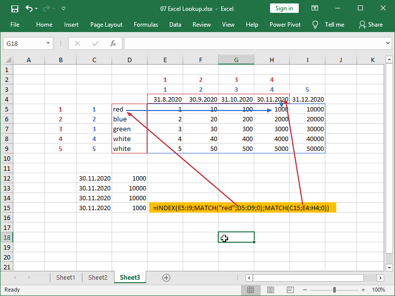
If we need to specify both row and column, we have to use two MATCH functions:

In this example, we are retrieving data from the cell range E5:I9.

The row from which data will be retrieved will be row 1 in that selection, as “red” matches row 1 of selection D5:D9.

The column from which data will be retrieved will be column 4 in that selection, as 30.11.2020 matches column 4 of selection E4:I4.

We can see that process more clearly here:

 

Make sure that the cell range in the INDEX function array has the same number of rows and columns as your lookup arrays and that they are correctly positioned.

Errors or incorrect results will be returned if the INDEX formula array and MATCH formula(s) array are not corresponding.

In the most common type of error, arrays are not aligned:

Arrays can also be of a different size:

If arrays are of a different size and start at the same position, the correct results can still be returned for the first part of the data not affected by error:

If arrays are of a different size and start at the same position, the correct results will not be returned for the second part of the data affected by error:

 

If we need to retrieve data from a single row, we can perform a simple horizontal lookup using the INDEX MATCH combination:

Note, we should set our row condition to 1.

 

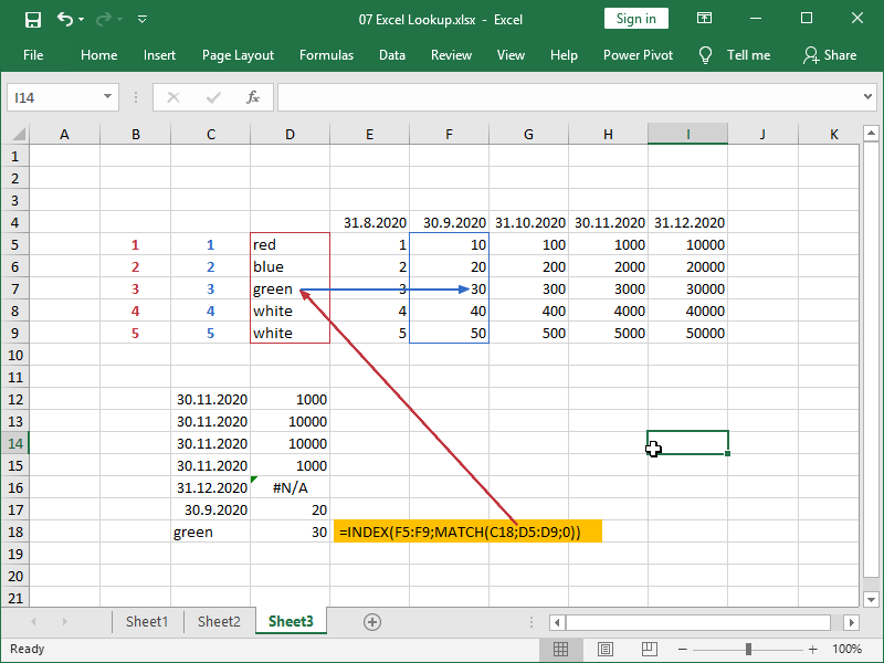
If we need to retrieve data from a single column, we can perform a simple vertical lookup using the INDEX MATCH combination:

Note, we could, but we didn’t have to set our column condition to 1.

 

You’ve probably already noticed that we have a double entry on our table; team white shows up twice.

What will happen when we try to look up “white”?

We don’t have an option to specify which match to use for the MATCH function. We will return the value corresponding to the first match, not necessarily the value we were hoping to return.

If our items are not unique, do we really need a match?

Do we need a sum? We can use the SUMIFS function if our items are repeating and we need a sum.

If we really need a second, third, or nth match, we can combine the IF function, the ROW function, and the SMALL function so that we can look up any occurrence of a specified item.

 

Retrieving data with unique identifiers

A unique identifier is a name that uniquely identifies an object within an identification scheme. In Excel, usually a name located in a table column that contains data in all of the rows, and that data is non-repeating.

Possible examples of unique identifiers are product codes (one code for every product), user IDs (one code for every user), usernames (one username per every user), email addresses (no double registrations with the same email address), and so on.

There could be several such columns with non-repeating data in all of the rows in any given table, i.e., the table containing the user ID will possibly also contain the email address, and they are both unique.

However, if we want to efficiently manage data in multiple large tables from multiple sources, we will usually select one unique identifier such as user ID (one code per every user), ensure that that code is non-repeating in our primary table (let’s call that table Users), and then ensure that this unique identifier is available in all other tables.

The combination of INDEX and MATCH functions is the preferred way of managing data structured in the way described in Excel.

 

Let’s now show this with a practical example.

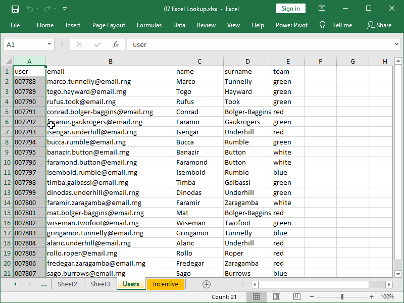
First, we have our table Users, with each user having its own unique ID:

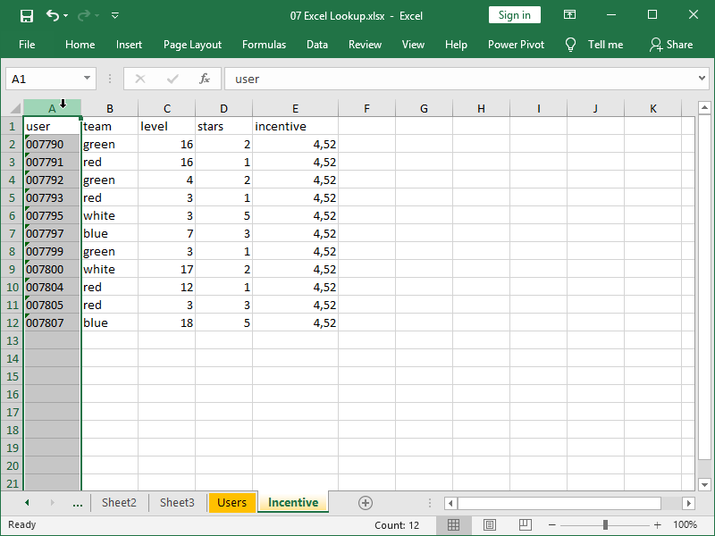
We also have our table Incentive, where we’ve also ensured that the unique IDs are available:

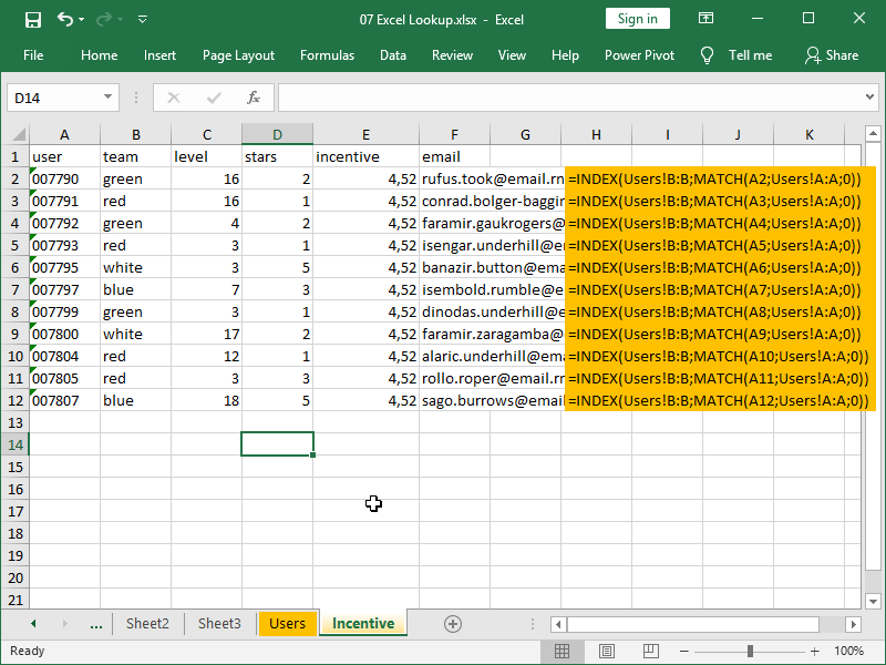
Let’s say we want to retrieve user email addresses. With INDEX MATCH, this is easy:

Here, we are matching users’ IDs with user IDs in column A, table Users. When a match is found, the value from the corresponding row in column B, table Users, is returned, i.e., the email address.

 

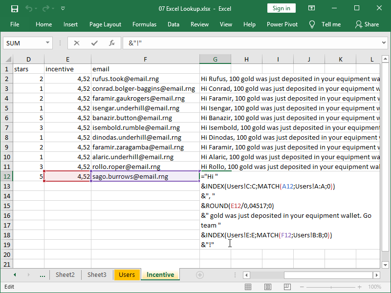
We can also use INDEX MATCH to generate text messages that users will receive:

Notice how we are retrieving parts of the message by matching both the user ID and, earlier retrieved, the email address with the table Users.

We can do this without errors as they are both unique in the Users table.

 

Notes:

If we need to perform a lookup with multiple criteria, see how to match multiple criteria in multiple columns.

Alternatively, the XLOOKUP function works much the same way as the INDEX MATCH combination as presented in this article, with slightly different syntax.