By combining FILTER with XLOOKUP, that corresponding array and/or filtering criteria can be returned from (un)related tables.
We can FILTER, and in the end, SUM, values based on criteria that are not present in the table we are returning values from.
In the following example, we will show how to use XLOOKUP in order to return filtering criteria:
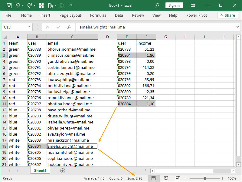
This table contains (repeating) user IDs and income related to those IDs.
The table to the left contains a mapping of those user IDs and user email addresses (both unique).
We are interested in retrieving a sum of values from the income column based on the email address of the user.
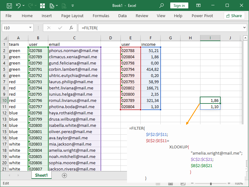
If we nest the XLOOKUP function as our filtering criteria, we can return the values we are interested in in a spilled array:
What is going on here?
We are trying to look up our input, the email address we are returning the values for, in the cell range $C$2:$C$21, and then retrieve the corresponding user ID from the cell range $B$2:$B$21.
That corresponding user ID is returned as a filtering criteria.
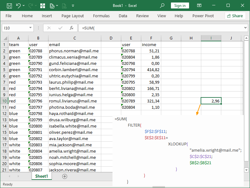
If we need a sum, we can additionally nest our formula in the SUM function:
In the following example, we will show how to use XLOOKUP in order to return corresponding arrays on which filtering criteria can be applied:
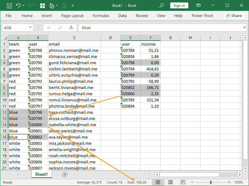
Again, this table contains (repeating) user IDs and income related to those IDs.
The table to the left contains a mapping of those user IDs (unique) and their related teams (non-unique).
We are interested in retrieving a sum of values from the income column for a particular team.
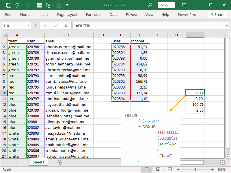
If we nest the XLOOKUP function as the source of the corresponding array on which filtering criteria will be applied, we can return the values we are interested in in a spilled array:
What is going on here?
We are trying to look up all of the user ID’s in the cell range $E$2:$E$11 with the user ID’s in the cell range $B$2:$B$21, and then retrieve the corresponding team names from the cell range $A$2:$A$21.
Finally, we are applying filtering criteria to the array of corresponding team names we’ve returned.
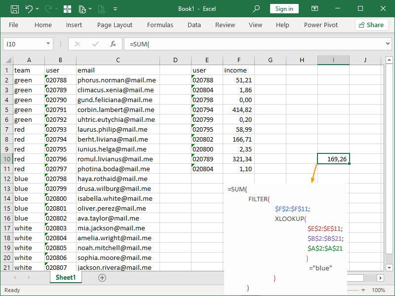
If we need a sum, we can additionally nest our formula in the SUM function:
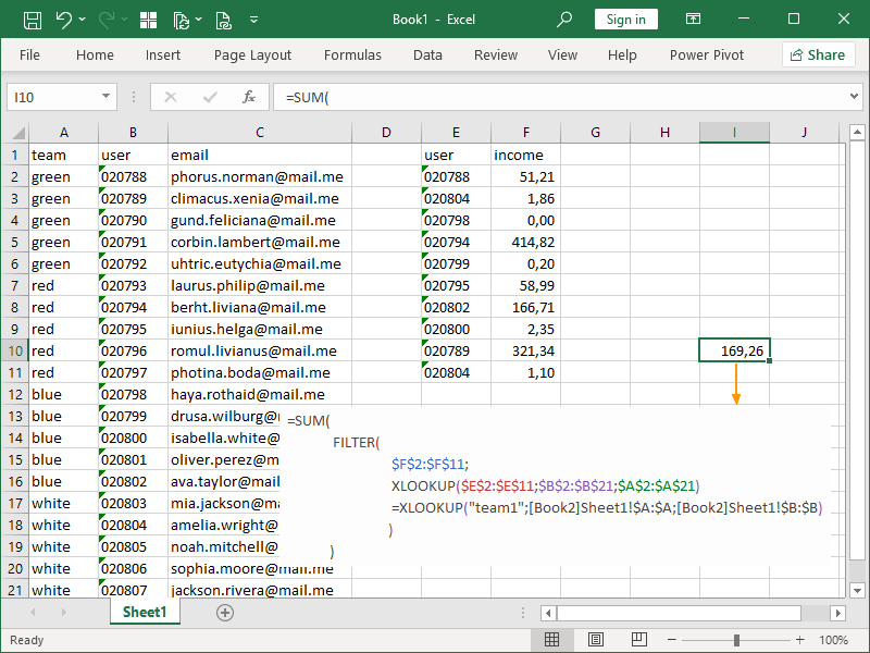
If needed, we can look up both the filtering criteria and the corresponding array to which filtering criteria will be applied:
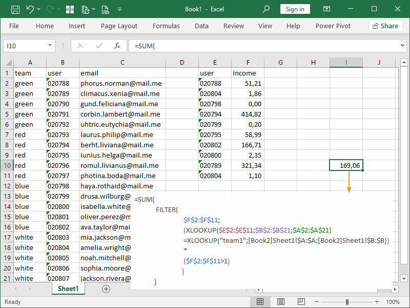
If needed, we can combine this type of criteria with other criteria:
Also consider the following example:
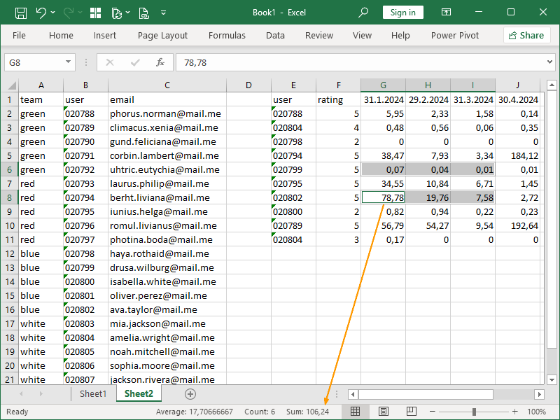
This table contains (repeating) user IDs, (repeating) ratings, and MTD income related to those IDs in several columns.
The table to the left contains a mapping of those user IDs (unique) and their related teams (non-unique).
We are interested in retrieving a sum of values from the selected columns for a particular team and rating.
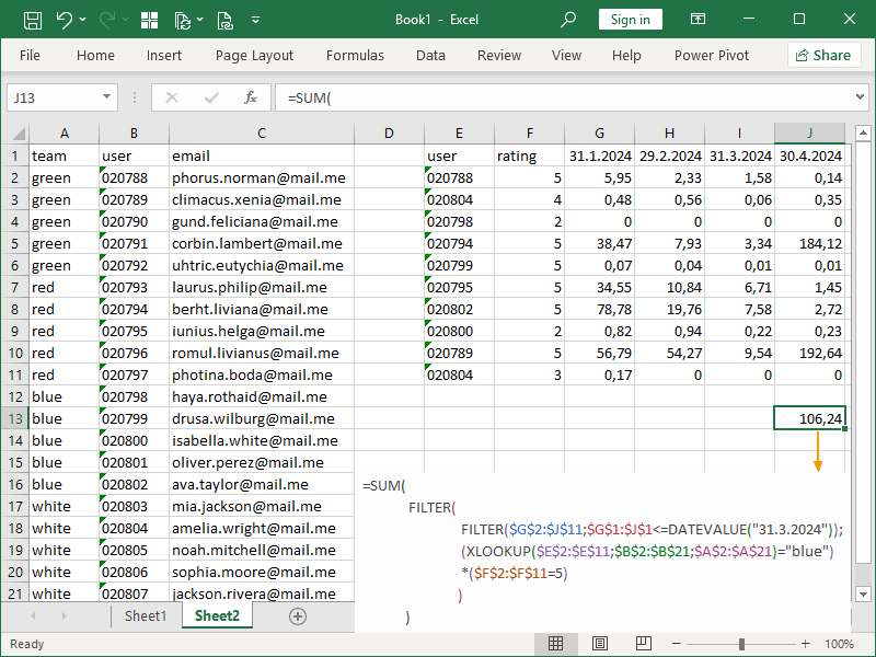
I.e., we need to sum all of the Q1 values for users that are members of the blue team and have a rating equal to 5.
We can accomplish this using already-shown principles; only now, our array to return values from will also be defined by another FILTER function:
Note, the already existing SUMIFS function adds all of the values that meet one or more criteria. The SUMIFS function can be extended in order to support the definition of a (single column or row) sum range in the function arguments and matched criteria if combined with XLOOKUP.
By combining the SUM, FILTER, and XLOOKUP functions, we are recreating and extending the SUMIFS function functionality further than the SUMIFS function can be extended. I.e., we can sum multiple columns, and we can use matched “criteria ranges”.
If you prefer the INDEX MATCH combination to the XLOOKUP function, see how to combine FILTER and INDEX MATCH in order to return the corresponding arrays and/or filtering criteria from (un)related tables.
Dig deeper:

5 thoughts on “Combining FILTER with XLOOKUP”