Using the SUMIFS function, we can sum all of the values in a defined column (or row) that meet one or more criteria.
SUMIFS criteria can reference cells, contain values or text, contain logical tests, or contain formulas and functions.
By nesting the INDEX MATCH combination or the XLOOKUP function as SUMIFS criteria, we can return values based on criteria that are not present in the table we are returning values from.
Consider the following example:
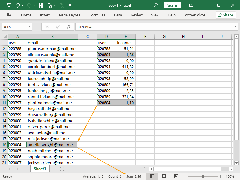
This table contains (repeating) user IDs and income related to those IDs.
The table to the left contains a mapping of those user IDs and user email addresses (both unique).
We are interested in retrieving a sum of values from the income column based on the email address of the user:
Also consider, we don’t want to use a helper column here.
Aside from avoiding extra work, helper columns are often not convenient or can’t be used for various reasons.
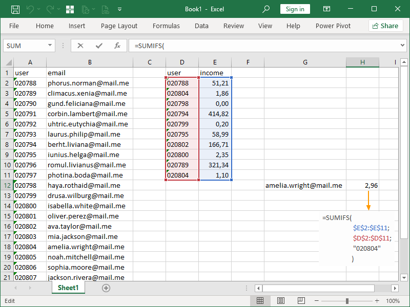
This is what it would look like if we’d retrieved our sum by manually entering the SUMIFS criteria:
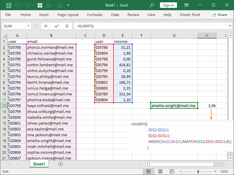
If we nest the INDEX MATCH combination as our SUMIFS criteria, we can retrieve our sum based on a related value:
What is going on here?
We are trying to MATCH our input, the email address we are returning the sum for, in the cell range $B$2:$B$21.
Using the INDEX function, we are retrieving the corresponding user ID from the cell range $A$2:$A$21.
That corresponding user ID is returned as criteria to the SUMIFS function.
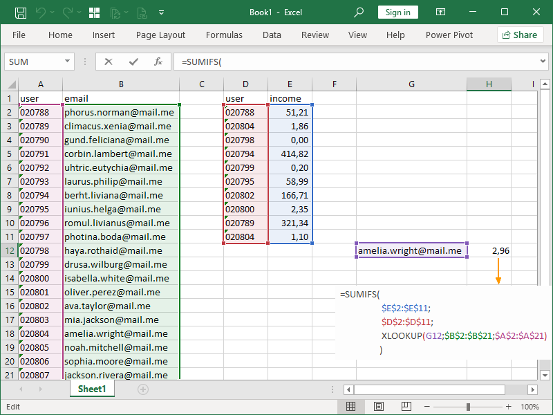
If we nest the XLOOKUP function as our SUMIFS criteria, we can also retrieve our sum based on a related value:
What is going on here?
We are trying to lookup our input, the email address we are returning the sum for, in the cell range $B$2:$B$21.
We are again retuning the corresponding user ID from the cell range $A$2:$A$21.
That corresponding user ID is returned as criteria to the SUMIFS function.
The basic principles shown here can be applied to other formulas as well. For example, you can combine COUNTIFS, AVERAGEIFS, MINIFS, MAXIFS, or even legacy functions such as SUMIF with INDEX MATCH or XLOOKUP in order to calculate values based on related values.
See also:
How to return the SUMIFS sum range using the INDEX MATCH combination
How to return the SUMIFS sum range using the XLOOKUP function
Dig deeper:
SUMIFS criteria: formulas, functions and conditional statements
Lookup with unique identifiers


3 thoughts on “SUMIFS criteria: INDEX MATCH or XLOOKUP criteria”