You will sometimes want to retrieve unique values from a data set, i.e., to find and remove duplicate values. While there are a few ways to do this, the most effective option is the Excel built-in feature Remove Duplicates.
The Remove Duplicates feature removes duplicate rows from the selected columns.
Duplicate rows are deleted in this process.
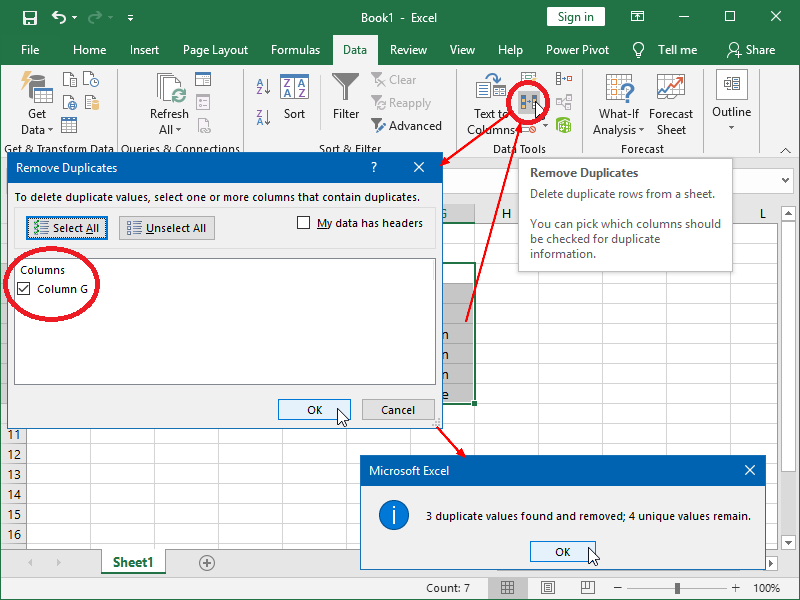
The simplest example of this process is the removal of duplicate values from a single column:
In this example, we’ve started with the data in column B. As we don’t want to destroy our original data, first we’ve copied our data to column G and then removed the duplicates.
Next, we’ve selected the data we want to remove duplicates from and followed the steps shown above.
Data that was deleted in the process is marked orange:
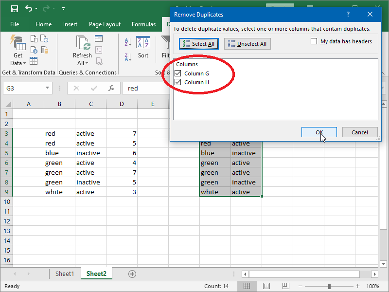
Removing data from multiple columns is very similar:
However, results are very different; notice that the third occurrence of the text “green” was not removed as the combination of “green” and “inactive” is unique:
Also notice that we once again first copied our data, and only then have we proceeded with duplicate removal. Had we not done so, our table would have been broken.
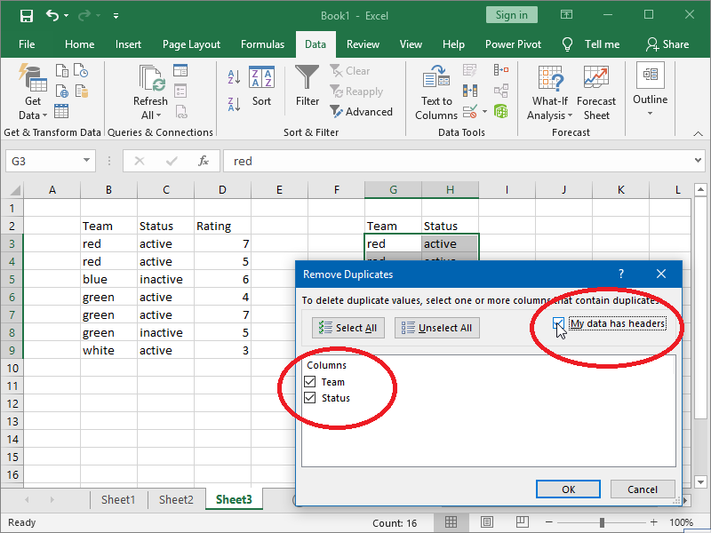
If your columns have headers, you can select the My data has headers option; however, this only does something if the value in your header repeats below the header, and you also want to keep it twice for that reason:
Selecting the whole columns and then using Remove Duplicates also makes little difference:
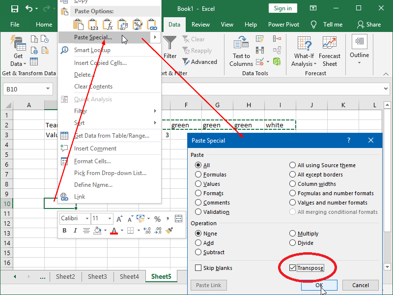
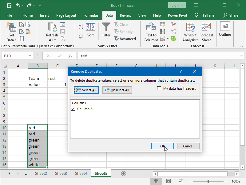
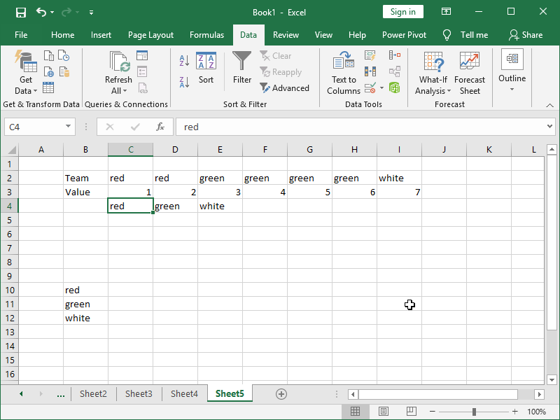
The Remove Duplicates feature does not support the removal of duplicate columns from the selected rows. If our data is structured in such a way, we will first have to transpose it.
We start by copying our data:
We next paste our data as Paste Special, Transpose:
We can then remove duplicates as usual:
If needed, we can Paste Special, Transpose it back:
The UNIQUE function replicates and extends Excel’s Remove Duplicates feature in formula form, allowing us to return a list of unique values in a list or range.
Dig deeper:





3 thoughts on “Remove Duplicates feature”