Excel Tables

What are Excel Tables?

Excel Tables, or just Tables, are tables superimposed over regular cells.

Excel Tables are assumed to be containing structured data.

Both tables and individual table columns are named and intended to be referenced in formulas by those names.

As they are typically used to load structured data from an external source into Excel, and that external data is typically accessed from Excel using the Data ribbon and then loaded into Table, they are also sometimes called Data Tables, even if that term is technically reserved for another object in Excel.

However, any existing range of cells can be formatted as a Table.

 

How to create or remove an Excel Table

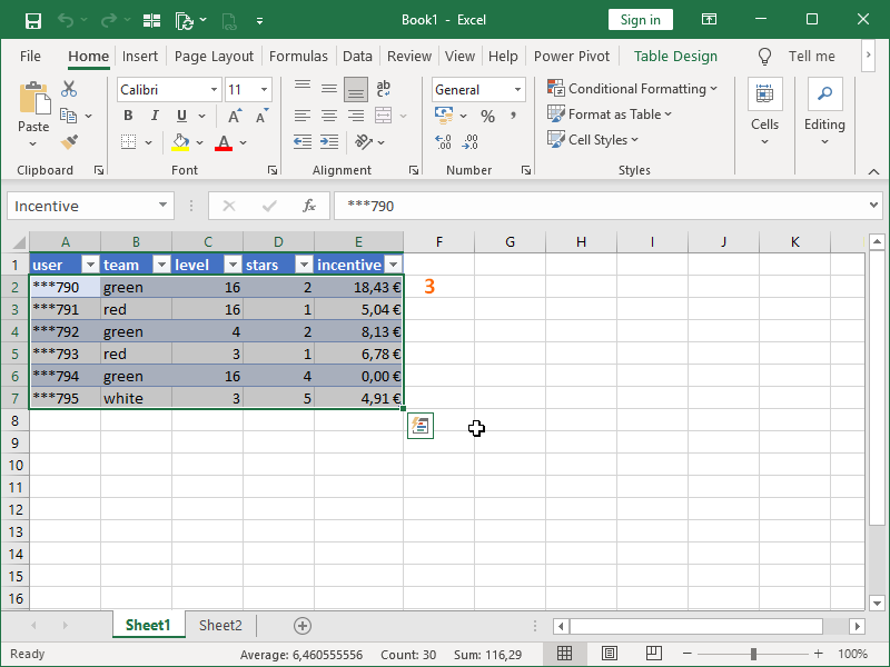
We can select any desired cell range and apply Format as Table to that range:

Once we format our cell range as a table, we can position ourselves in any part of that table and a new ribbon, Table Design will become available:

In general, in order to modify an existing Table in any way, you will have to be positioned inside of that table.

 

It is also worth distinguishing between the table itself and the table style.

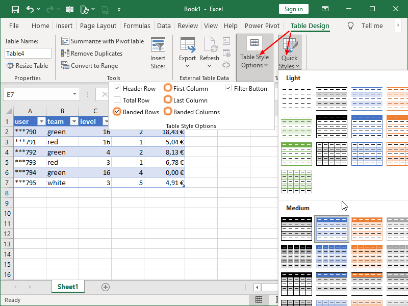
Excel Tables are by default rather colorful, and the rows are banded so that the data is better distinguishable.

Those styles can be modified in the Table Design ribbon, Quick Styles (style can be changed), and Table Style Options (banding of rows can be turned off, banding of columns can be turned on, first or last column can be bolded):

 

However, if we want to remove our table, this is can be done with the help of the Convert to Range button. Data is converted to a range but the formatting remains.

Vice versa, if we remove the formatting, the table itself will remain.

Those are two separate actions, and both can be done without the other one being done.

Hence, in order to completely remove the Table, we have to do both:

 

How to remove Excel Table connections

When data is loaded into an Excel Table from an external source, we have to distinguish between the connection to the external data source on the workbook level and the loading of that data into the Table itself.

We can stop future updates of Excel Tables (data refresh) with the help of the Unlink button:

The Unlink button will not convert the table to a cell range or remove the formatting.

However, if we are converting a table to a range, the Convert to Range action described above will by definition also stop future updates as Table will no longer exist.

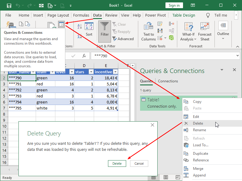
In both cases, the now inactive connection to the external data source will remain in our workbook. If it is not needed, it can be removed in Queries and Connections:

 

Excel Table Names

Generic Table names are generated when Tables are created (Table1, Table2, etc.)

Those names are visible in the Table Design ribbon. They are easy to change, and in principle, should be changed in order to represent the data available:

 

All available Tables in a workbook will be present in the Name Box. This can be used in order to navigate to a table:

Once a table name is selected, we are led to the desired table:

 

Table column names are also generated when Tables are created.

If the “My table has headers” option is selected, as it was in our example, they are taken from the first row of selected cells.

If the My table has headers” option is not selected, generic names are given (Column1, Column2, etc.).

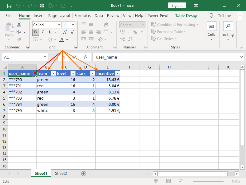
In principle, if a table is used to load external data, column names should not be messed with. However, if needed, they can be changed directly in the Header Row:

Column Names in Excel Tables will always be text stings.

If a date or any other type of number is being used as a column name, it will be converted to a text string. Those numbers formatted as text can cause issues with matching (lookup).

 

Excel Table Components

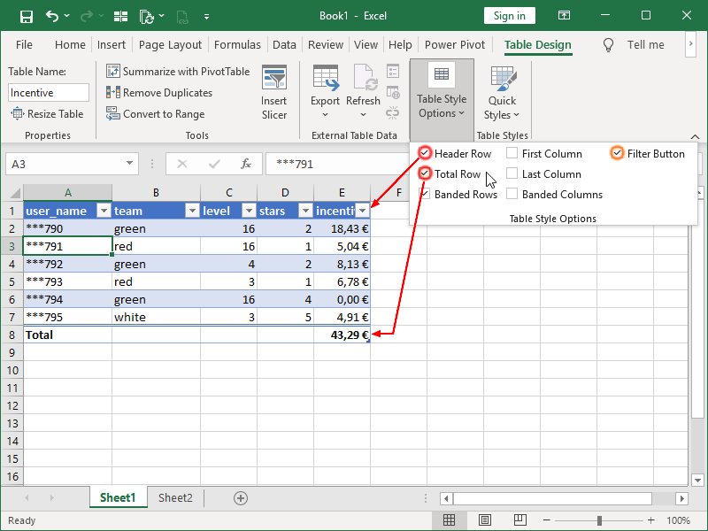
Each Excel Table will contain:

• Data, in one or more rows.
• Headers, with Header Row being turned on by default, can be turned off if desired.
• Totals, with Total Row being turned off by default, can be turned on if desired.

Filter buttons will be located in the Header Row, turned on by default, and can also be turned off if desired.

Total Row can actually be customized and totals can be created for all columns. Each Total Row cell can contain a function calculating some kind of total.

The default options offered are based on the SUBTOTAL function (filtered out values will not be accounted for in the total row), but any function can be manually entered:

 

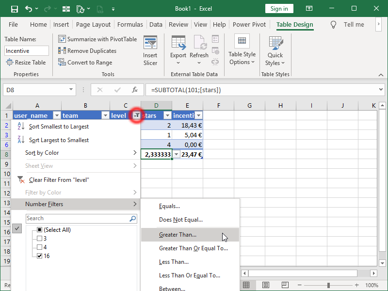
Filter buttons will offer all of the typical Sort & Filter options:

Note the changes in the totals.

 

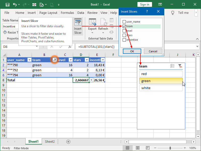
Filtering can also be done via slicers:

Again, note the changes in the totals.

Also note that, when the slicer is in use, the filter button is also active.

 

Dynamically updated Calculated Columns

We can insert (delete, select) table columns by positioning ourselves on the desired location in the table, right-clicking and selecting Insert Table Column (to the Right):

 

We can manually rename those table columns or enter values into them as we please:

 

It is different with formulas.

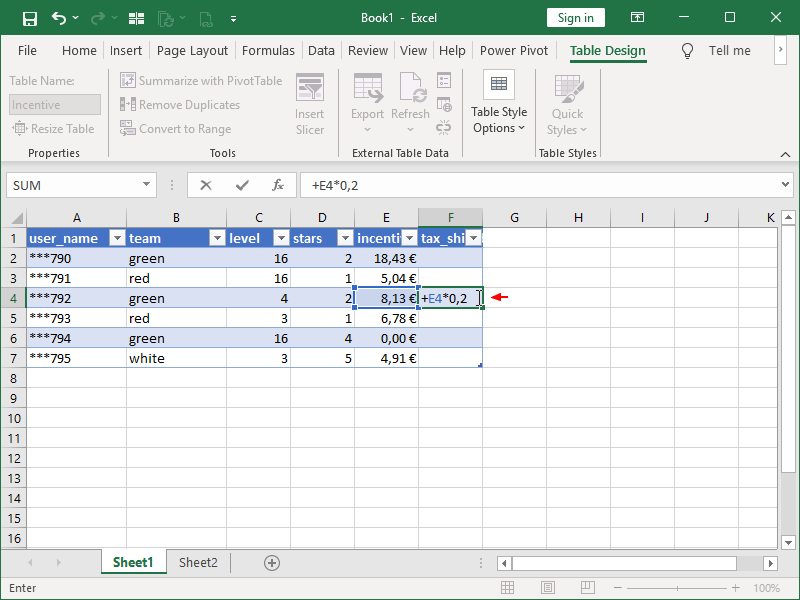
By default, any formula entered in any single cell is automatically expanded to the rest of the column.

We can start by entering a formula into any cell of the column:

And that formula is automatically expanded when we press the Enter button:

 

When a formula is changed in any row of the column, that update will also expand to the rest of the calculated column:

 

If you enter a formula, and it expands, those are two steps to potentially Undo.

If, for some reason, you want to have a different formula for a specific cell of the Table, you can enter it, and after it expands, use just one Undo.

 

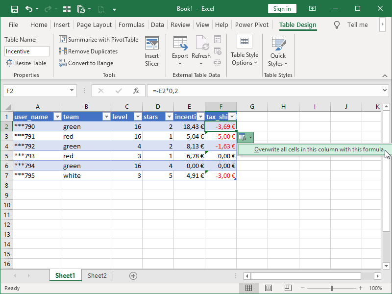
If our column is a collection of different formulas and/or values, we can override that and apply a single formula to the whole column by (re)entering the correct formula and applying the following option:

 

If we expand our table with additional rows, our calculated columns will also expand.

That will happen if we enter or paste data directly below the table, or if our linked table contains more rows after refresh.

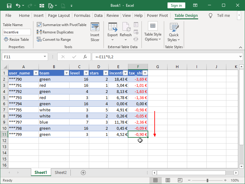
Consider the following example, we intend to paste new rows under our current table:

Momentarily, those rows are formatted as part of the table, and the calculated column formulas are expanded:

As we are pasting data instead of refreshing an external connection, if needed, in this case it would be possible to use one Undo to remove the automatic expansion of the table and calculated columns.

 

Structured references in Excel Tables

Structured references are references to tables and table column names, in contrast to references to cell ranges.

They are the intended way of referencing data from Excel Tables due to their presumed advantages (“human readable” references, structured references adjust automatically when data is added or removed from the table, or when columns are renamed).

 

Structured references can contain:

Table name, if a table is referenced from outside of the table (qualified reference). If we are using structured references inside of a table, we don’t have to name that table (unqualified reference).

Column name, enclosed in brackets.

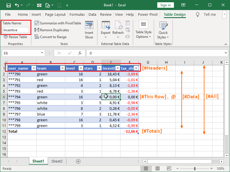
Item specifier (#All, #Headers, #Data, #Totals, #This Row), which is used only situationally, and, if used, is also enclosed in brackets. If no specifier is used, only the data part of the table is referenced, headers and totals are not.

The only case in which an item specifier is often used are references to single rows, and then a shorter @ specifier is used.

This image shows all the names and specifiers we can use:

 

In the following example, we are referencing a single row:

The automatically expanded formula from the G5 cell contains only column names enclosed inside of the brackets. These are unqualified references.

The formula in the cell I7 first references the table name, and then the column names enclosed inside of the brackets. These are qualified references.

The formula in the cell I14 is returning an error, as there is no data in our table in that row.

 

Note the different ways columns incentive and tax_shield are referenced.

Double brackets are required when special characters are present in column names. When brackets or a number sign are present in a column name, a single quotation mark can be used as an escape character.

 

When referencing a whole table column (data part), we are writing our formulas in this way:

Incentive[[#Data];[net_incentive]]

This can be shortened to

Incentive[[net_incentive]]

This can (and will be automatically in this case) be shortened to:

Incentive[net_incentive]

 

Considering the following usage of structured references in the SUMIFS function:

 

However, if we drag that formula to the right, it will be automatically adjusted in the following way:

In a sense, those references are “not locked”.

 

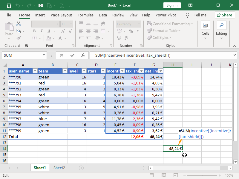
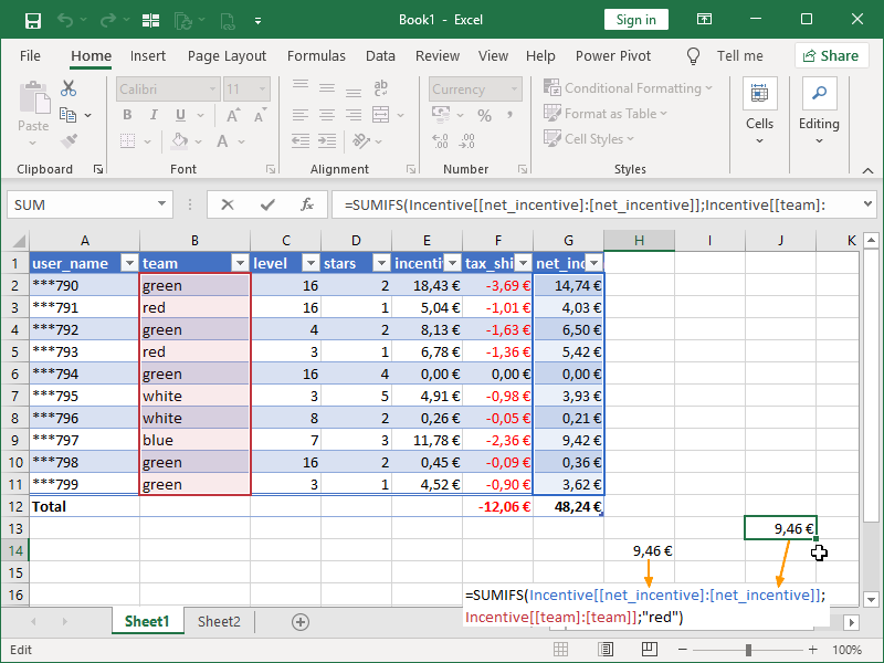
If we want to reference two or more columns, we can do that by using the range operator (colon) inside of multiple brackets:

 

We can use that way of writing formulas in order to “lock” structured references to columns in an Excel Table, as those are not moving:

 

References to Tables located in external workbooks will look something like this:

Book1.xlsx!Incentive[net_incentive]

However, problems with formula updates and other issues can occur. Structured references are, after all, intended to be used inside of Excel Tables, or to reference Tables located in the same workbook.

Retrieving data from Tables in outside workbooks is still better done via references to cell ranges those tables are superimposed over.