Both the MATCH function and the XLOOKUP function look only for the first (last) available match in the array.
This is perfectly reasonable in most cases, as we are expecting to deal with unique identifiers when looking up data. However, sometimes we will have to look up the second, third, fourth, or nth value.
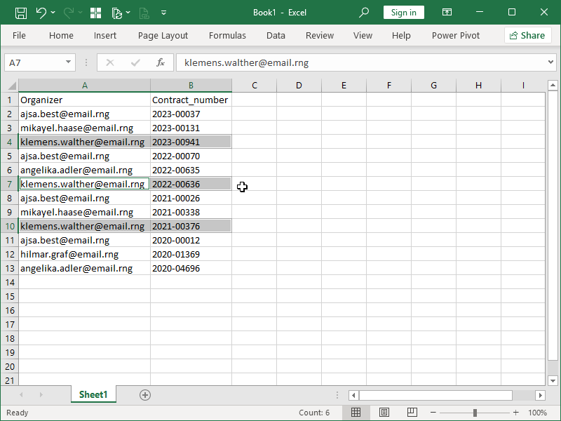
Consider the following example:
Our table contains a list of contract numbers in column B and contact email addresses in column A. Contract numbers are unique; however, email addresses are not, and in this particular example, an email address repeats three times.
If we want to look up the second contract number for the marked email address, how can we accomplish that?
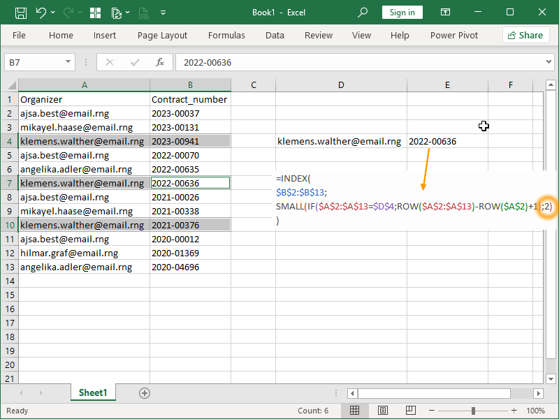
As the MATCH function doesn’t support this type of lookup, we will combine the IF function, the ROW function, and the SMALL function so that we can look up any occurrence of that item:
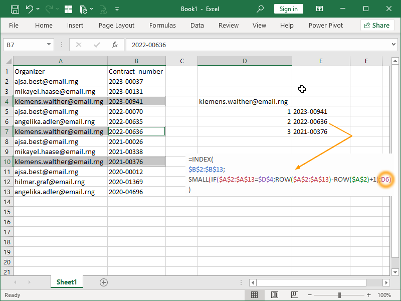
We can also look up all three occurrences of that item:
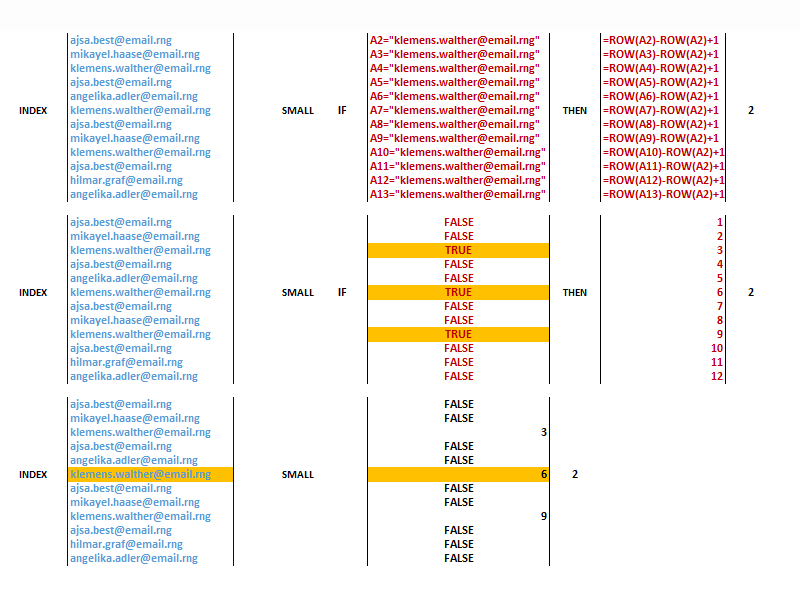
What is going on here?
In our first array nested inside the IF function, we are checking whether the email address in column A equals the email address we are trying to match.
If the email address matches, we will return the row number of the match. The row number we are returning is the row number inside the array, and we are calculating it by retrieving row numbers using the ROW function and then deducting the row numbers not in the array also using the ROW function.
We can then use the SMALL function to retrieve the first, second, or third smallest row number. Parts of an array that consist of FALSE values are helpfully ignored by the SMALL function.
The number returned by the SMALL function is the row number we are using as the row number part of the argument for the INDEX function.
Alternatively, in the newer versions of Excel, we can also use the FILTER function in order to retrieve the 2nd, the 3rd, or the nth value.
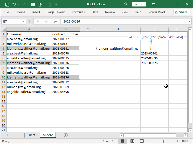
The FILTER function returns all records for the defined criteria:
Depending on what we are trying to accomplish, even this by itself can be enough.
However, if we specifically want to return the 2nd, the 3rd, or the nth value, we will need to combine INDEX with FILTER.
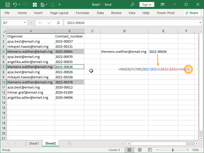
By nesting the FILTER returns into the INDEX function, we can return the 2nd match:
Note the difference in approach.
The array we are returning data from here is not an array of cells located in column A, but the return of the FILTER function visible in the previous example.
See also:
Combining multiple arrays into a single lookup array
Dig deeper:
Lookup with unique identifiers

7 thoughts on “Lookup the 2nd, the 3rd, or the nth value”