
If we have to look up items in tables where we can’t use unique identifiers (there are no names located in a table column that contains data in all of the rows, and that data is non-repeating), we will probably have to resort to matching multiple criteria in multiple columns.
This approach is described in this article.
However, in modern versions of Excel supporting dynamic array formulas, we can also use a much simpler approach – we can combine multiple arrays (or combine multiple cell ranges into a single spilled array) in order to generate a single lookup array.
Consider the following example:
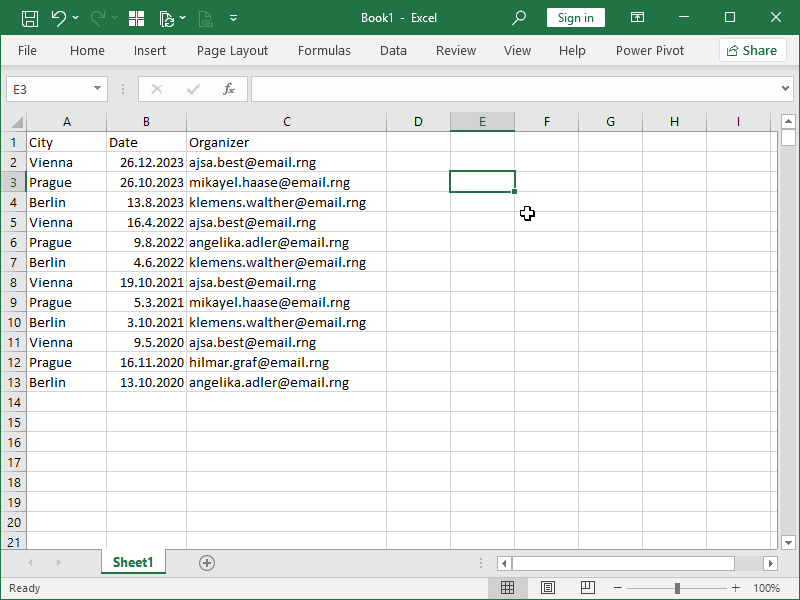
Each year, multiple game tournaments are held in repeating cities, organized by various repeating organizers. Items in the column City are not unique, nor are they in the column Date or the column Organizer.
What is unique in this combination are the City and Date combinations.
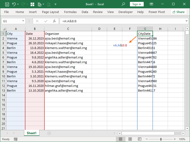
It is trivial to combine those two columns into a single array:
Given that we are dealing with dates here, we will also have to format them as text using the TEXT function in order to make our lookup easier:
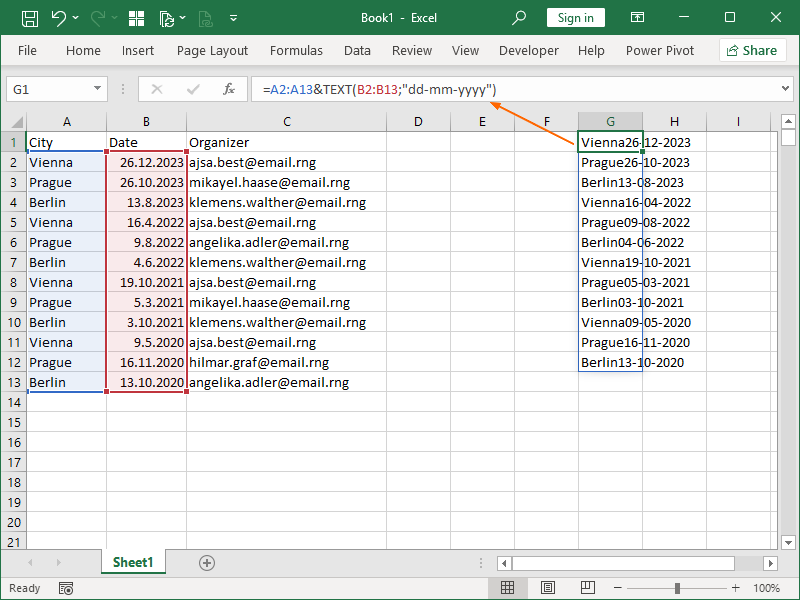
Note, we can’t perform this operation on the whole column B, as the value in the cell B1 is already text and not date.
Knowing what we now know, how can we retrieve the organizer email address for the tournament held in Prague in 2022?
We can look up Prague and 2022 in our spilled array in the following way using the INDEX MATCH combination:
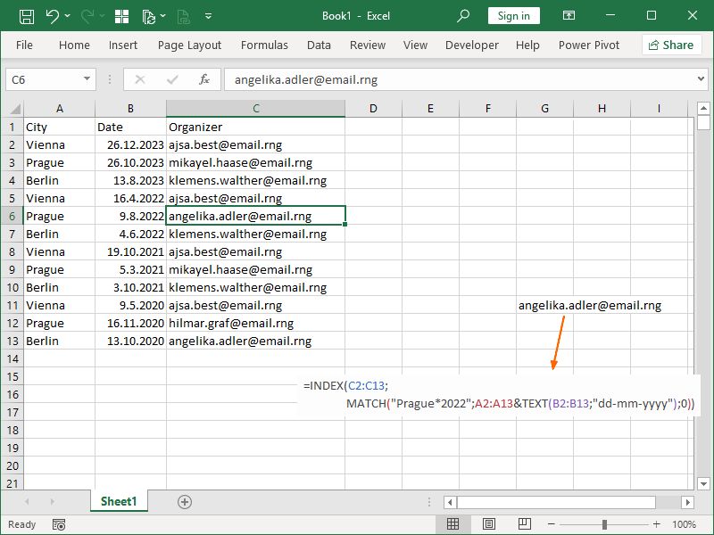
We are performing a partial match using an asterisk * here instead of searching for the full string to simplify things here.
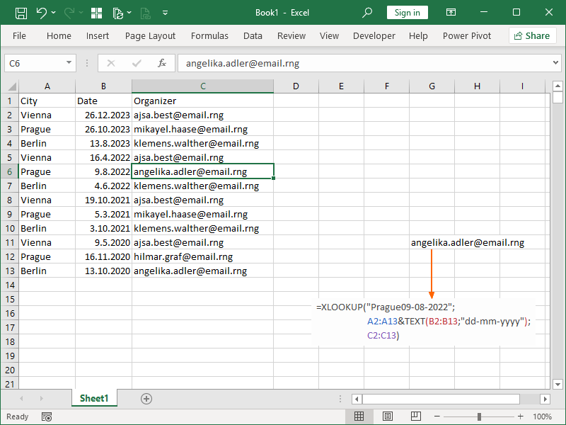
Searching for the full string “Prague09-08-2022” would return the same result, as we will show in the next example.
We can look up Prague and 2022 in our spilled array in the following way using the XLOOKUP function:
What would happen if there were two or more matches, i.e., two or more tournaments organized in the same city in the same year?
Both the INDEX MATCH combination and the XLOOKUP function look only for the first available match on the list, and only the first available match would be returned.
The FILTER function can also be used to achieve the same results as shown here, either by using the shown approach of combining multiple arrays or without it. As the FILTER function by default spills all available results, 2nd, 3rd, etc. matches would be spilled to the cells towards the bottom.
In order for the function to be able to use arrays resulting from combinations (or, to be more precise, in our example, we are combining two cell ranges into a spilled array), it has to be able to use arrays as part of the argument in the first place.
As already demonstrated, INDEX, MATCH and XLOOKUP function can use arrays in such a way. However, SUMIFS and related functions can’t.
Dig deeper:
Lookup with unique identifiers
How to return values adjacent to the looked-up values
One thought on “Combining multiple arrays into a single lookup array”