With conditional formatting, among other things, we can join indication icons to our numbers.
While we can rearrange available icons as we wish, the choice of available icons is fairly limited:
In particular, while Green Arrow Up and Red Arrow Down are available, we don’t have the often-requested Green Arrow Down and Red Arrow Up.
We can expand our choice of icons with the help of the Wingdings fonts, a series of fonts that render characters as a variety of symbols.
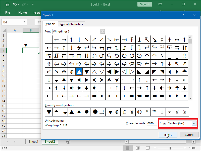
For this purpose, we can use either the symbols from the Wingdings, or from the Wingdings 2, or from the Wingdings 3 font, but not combinations. Wingdings 3 is particularly useful for this task because it contains mostly different forms of arrows and triangles. You will also have a hard time identifying some of the characters behind the symbols if you don’t select the Symbol (hex) option:
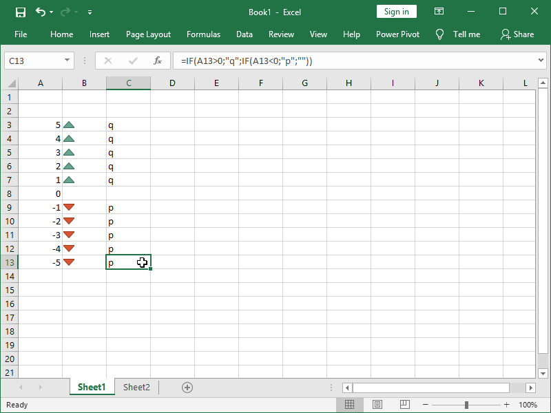
Cell B3 actually contains the character “q”, while cell B4 actually contains the character “p”. You will see those characters in the formula bar if positioned on the cell:
Now that we know that, we can then return either the character “q” or the character “p” with the help of the IF formula:
We can next format the cells containing those characters as Wingdings 3. We can also use green as the default color in order to speed things up:
We will finish our job with the help of Conditional Formatting:
We will format only those cells that contain the character “p”:
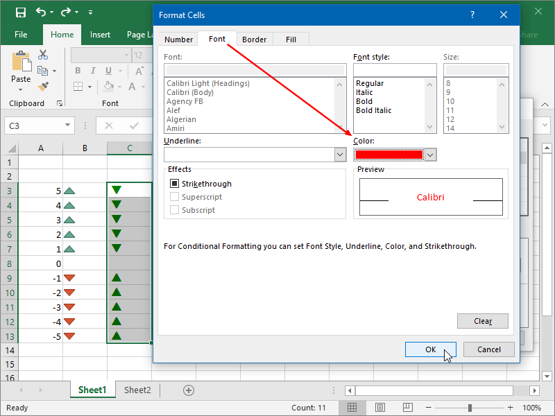
The text should be colored red in those cells that contain the character “p”:
Once we apply our Conditional Formatting, our custom Green Arrow Down and Red Arrow Up icon set will be up and running:
Following these principles, we can, if needed, use multiple Wingdings characters as our indicators.
We can format any of them into any desired color with the help of the “Format only cells that contain Cell Value equal to” rule.
Dig deeper:


