
In general, a lookup function such as the XLOOKUP function searches a corresponding range or an array for a match and returns the matching item from a range or array.
If our data is structured in a way that we can’t search for a match in a corresponding array (but the data still is structured), a typical lookup function will not be able to help us. However, the INDEX MATCH combination still can.
Remember, the INDEX function returns the value from a range of cells based on the row and column specified in the function arguments.
The syntax of the INDEX function is as follows:
= INDEX ( array ; row_num ; column_num )
The row number is always an integer, such as 0, 1, 2, 3,…
A column number is always an integer, such as 0, 1, 2, 3,…
It doesn’t matter how we set or calculate those row and column integer numbers (and if we input decimal numbers, they will be rounded down to integer numbers anyway).
Typically, we will return those row and column numbers using the MATCH function, which returns the relative position of the item in the range in the form of an integer number. However, nothing is stopping us from performing additional operations with those numbers.
Consider the following example:
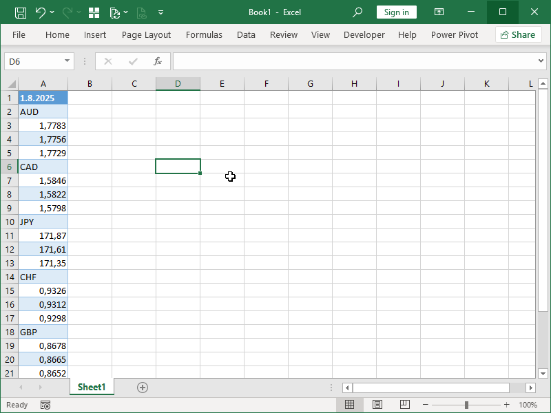
Every day, we are receiving a data dump with the exchange rates for the previous day. We need to retrieve the CHF selling rate from this data. The data will always be structured in the same way: first the currency code, then the buying, middle, and finally the selling rate.
The easiest way to retrieve the CHF selling rate from this data is to MATCH the CHF code and move three rows below, which can easily be achieved using the INDEX MATCH combination:
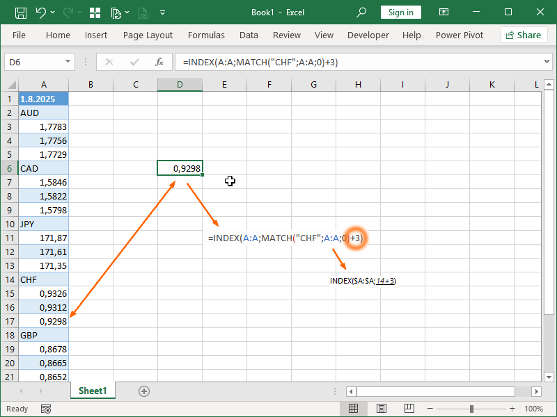
Here, we are using the MATCH function to return the position of the string “CHF” in column A and then moving three rows below by adding 3 to that position.
Now consider the following example:
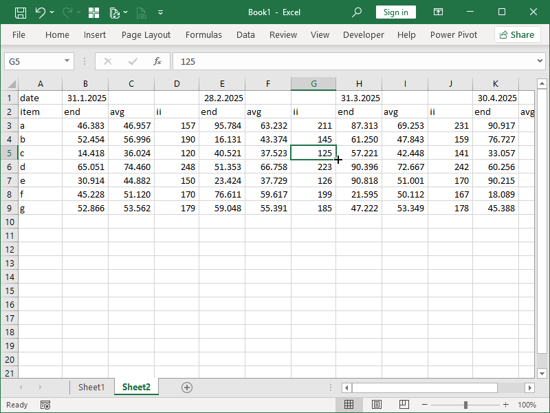
Every month, we are receiving a data dump with the end volumes, average volumes, and interest income values for the last n months. We need to retrieve the interest income for product c, for February, located in the cell G5.
The data will always be structured in the same way, with the first row containing end-of-month dates and the second headers for the end volumes, average volumes, and interest income values, always in that order.
However, dates in the first row are only present above the end volumes. We cannot look up with multiple criteria here.
What we can do, however, is to match those dates. Given that the interest income is always two columns to the right of the column containing the end-of-month date in the first row, we can simply add 2 to our MATCH return:
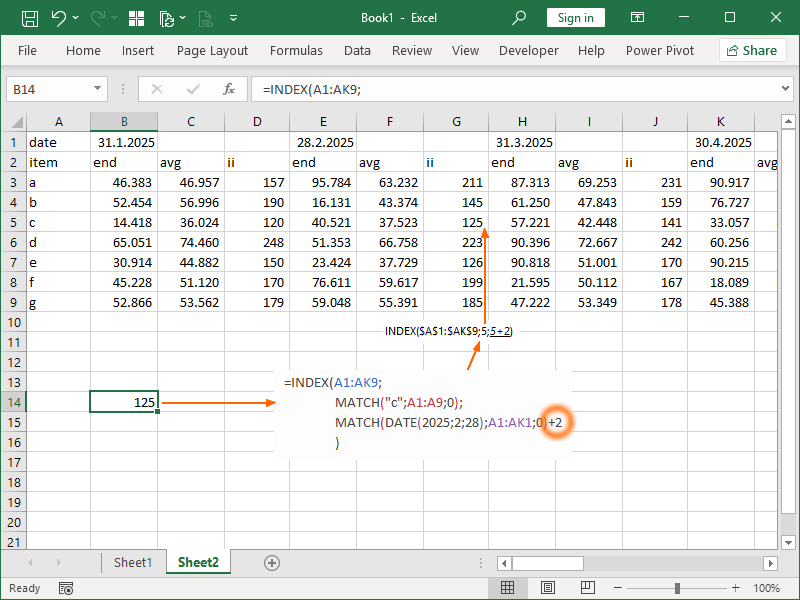
Here, we are using the MATCH function to return the position of the string “c” in the cell range A1:A9.
We are also using the MATCH function to return the position of the 28th of February in the cell range A1:AK1, and then moving two columns to the right by adding 2 to that position.
In the end, we will return the value from the 5th row and 7th column in the cell range A1:AK9.
Dig deeper:
2 thoughts on “How to return values adjacent to the looked-up values”