You will sometimes need to make some of your numbers appear invisible.
In this text we will show how to accomplish this goal using a custom number format, as we want to avoid the commonly used white font color and other problematic methods of accomplishing this goal.
Consider the following example:
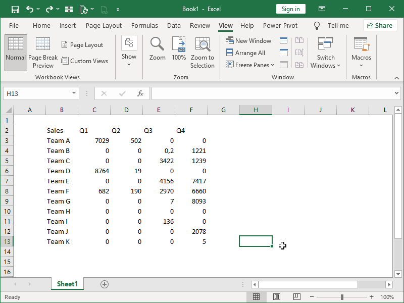
This is a table that will be linked into a PowerPoint presentation, and the gridlines are not shown.
Multiple cells contain zeros. We want those to appear invisible in order to make the table cleaner.
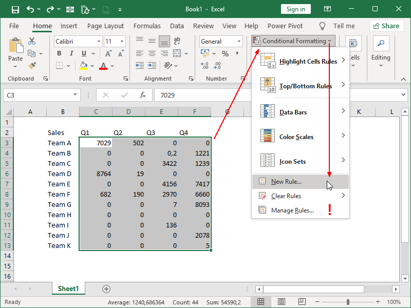
We can apply a new (or modify an existing) conditional formatting rule via the Home ribbon:
We will use the “Use a formula to determine which cells to format” rule type:
Our formula should use relative references, as shown above.
With our formula, all selected cells in Sheet1, which contain values equal to zero, will be formatted.
We will set up our format via the Format Cell window:
We should apply a custom number format to those cells, and that number format should be two consecutive semicolons, as shown above.
Our table now doesn’t show us the numbers that are equal to zero, those numbers are still there, but now invisible:
In PowerPoint, our table will now look like this:
Note that we are actually not using these definitions here as intended. We are instead just specifying a number format where the number is not shown, whether positive, negative, or zero. Using conditional formatting, we’ve already specified that this custom number format will be applied only to zeros.
Using this approach, we are not limited to invisible zeros, positive or negative numbers – we can keep hidden any specific number, any range of numbers, or any numbers outside of a defined range.
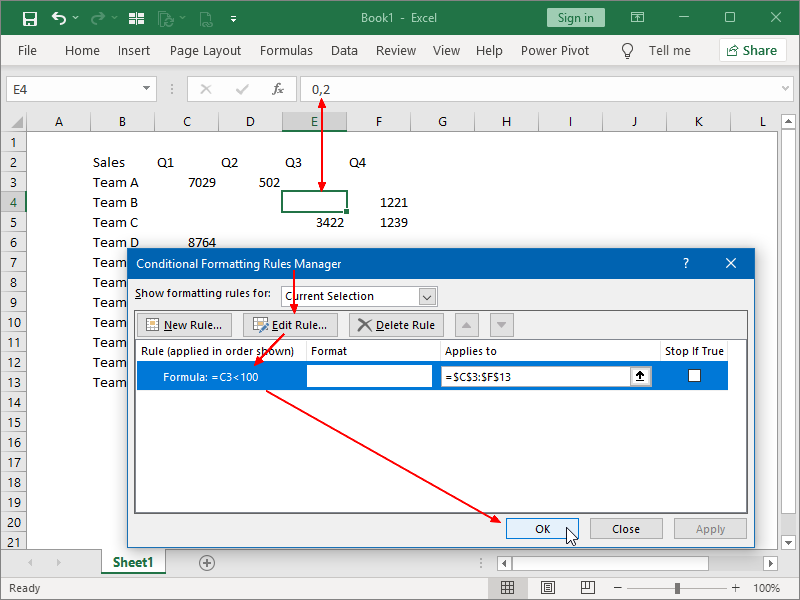
For example, we could modify our conditional formatting rule in order to not show numbers smaller than 100:
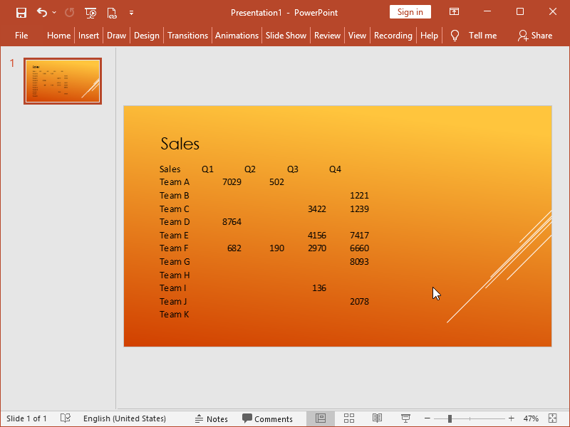
In PowerPoint, our table will now look like this:
Dig deeper:
Automated presentations – linking of Excel data to PowerPoint


One thought on “Invisible Numbers with Conditional Formatting”