
What are Pivot Tables?
Pivot Tables are aggregations of groups of values from more extensive data sets (cell ranges, Excel Tables, external databases, etc.) that contain structured data.
Pivot tables are objects superimposed over regular cells. They will usually contain row, column, and value fields. Those can easily be added, removed, rearranged, or modified.
While Pivot Tables can be used for many purposes, their primary use case is to help us quickly slice and analyze large and/or unknown data sets and recognize patterns and locations of desired information.
How to create or remove a Pivot Table
Consider the following example:
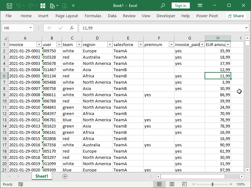
Here, we have a large amount of structured data in our cell range. We can do some basic analysis using filters, but given the large amount of rows, this is not very effective.
However, we can insert a Pivot Table by first selecting that data and then clicking on the Pivot Table button located on the Insert tab:
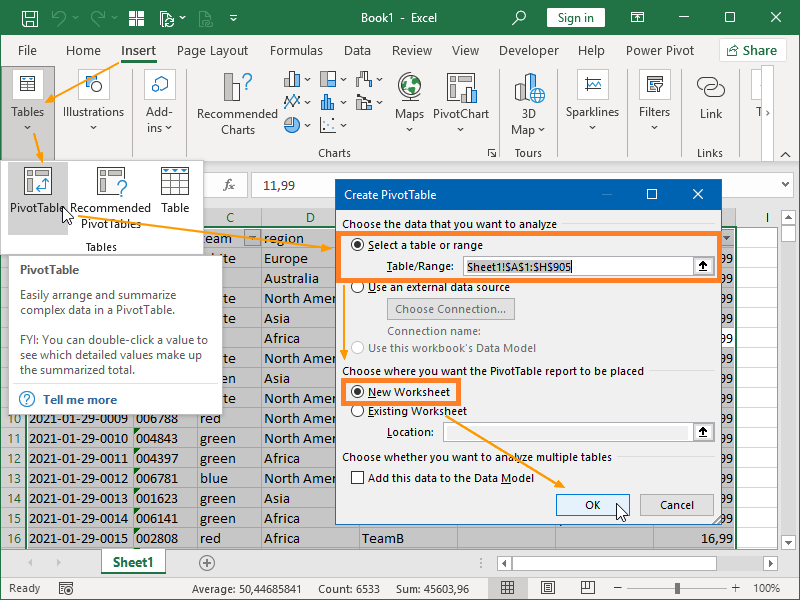
Given that we have previously selected our data, our data source, in this case cell range, is already defined. Had we not done so, we would have to select it in this step, either from a Table/Range, external data source, or Data Model.
By default, new Pivot Tables are inserted into new worksheets, but we can also specify an already existing location within a workbook.
Our newly inserted Pivot Table will appear in a new worksheet, and if we click on it, to the right, Pivot Table Fields window will appear, with two new tabs, PivotTable Analyze and Desing also appearing:
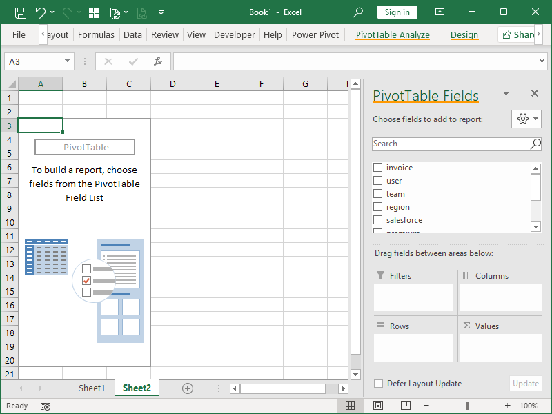
While the Design tab will contain commands for changes in the appearance of the Pivot Table, the PivotTable Analyze will contain commands for everything else, including the command that toggles the PivotTable Fields window on and off.
We can remove unwanted Pivot Tables by selecting all the cells superimposed by the Pivot Table and deleting them:
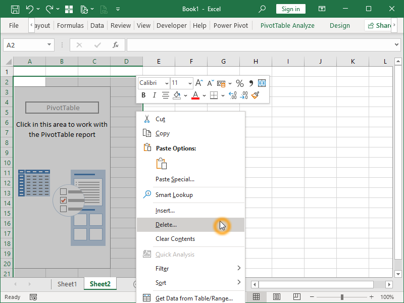
Alternatively, we can also use copy and paste to remove the table while keeping the generated aggregations.
How to change Pivot Table Data Source
If our source data updates, we can update our Pivot Table by using PivotTable Analyze / Refresh / Refresh.
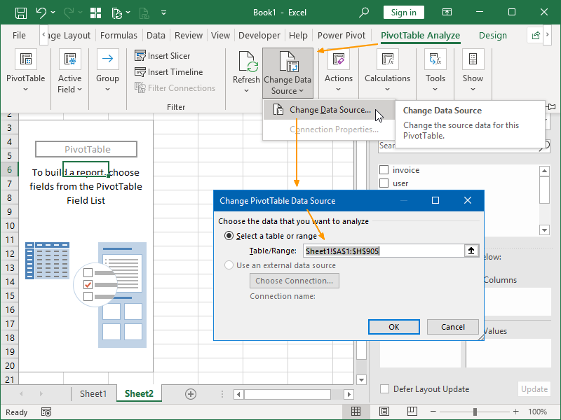
If we want to change the source data, we can do that by using the Change Data Source command located next to the Refresh command:
Pivot Table Fields: Values
If our source column contains values, it can be added to the Pivot Table Values area:
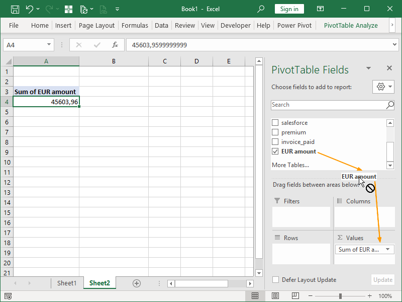
For columns containing numbers, the sum of the values is the default.
For columns containing text, the count of the values is the default.
This can be (if applicable) changed in the Value Field Settings:
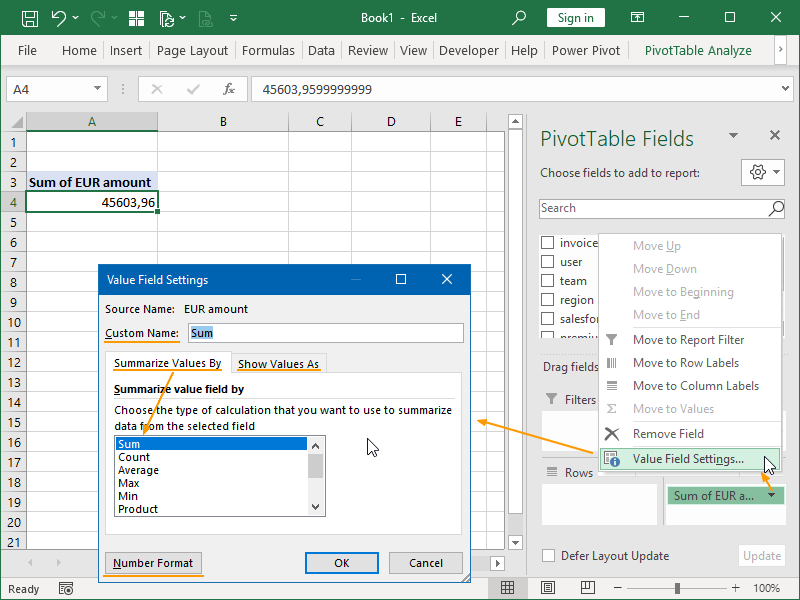
Multiple fields can be added to Values. The same field can be added to Values multiple times!
Here, we have again added the same field to Values:
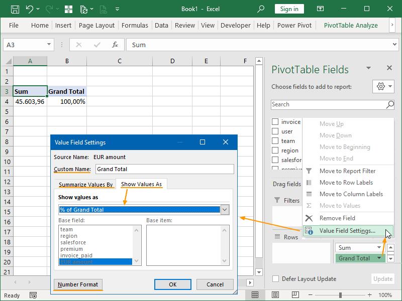
As visible, under Show Values As, we can also set up some calculations – % of Grand Total, % Of, Difference From, Rank, etc. In this example, we have changed this from No Calculation to % of Grand Total.
We have also renamed this value to Grand Total – we have done this by entering a value in Custom Name.
We can also change the applied number format by using the Number Format command. If needed, using this command, we can also apply a custom number format; for example, our numbers could be formatted to be shown as thousands or millions.
Pivot Table Fields: Rows and Columns
We can drag items from Fields to Rows and Columns in whatever order it suits us:
Once dragged, they can also be (re)arranged as we want.
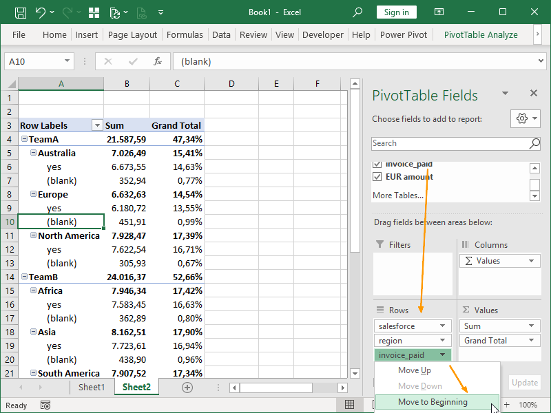
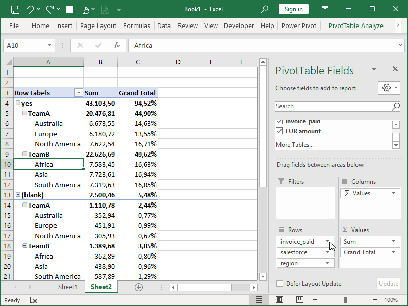
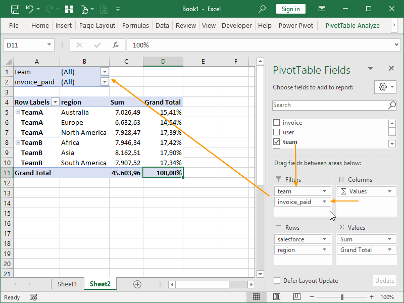
If we move invoice_paid to the beginning, our PivotTable also restructures:
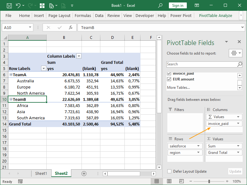
We can also freely move our fields between Rows, Columns, Filters and Values.
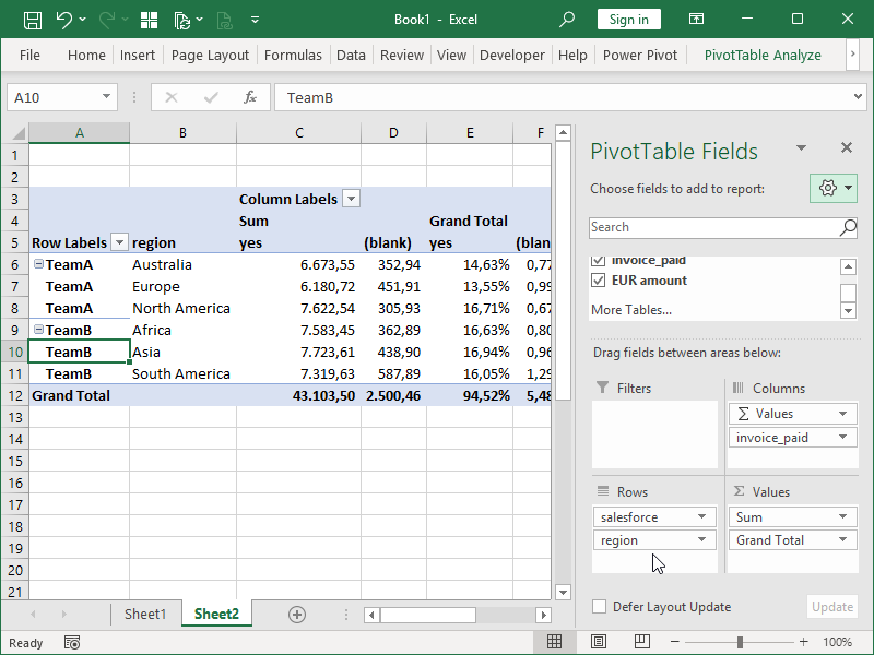
In this example, we have moving our invoice_paid field to Columns:
With Rows and Columns, we will have Field Settings command available:
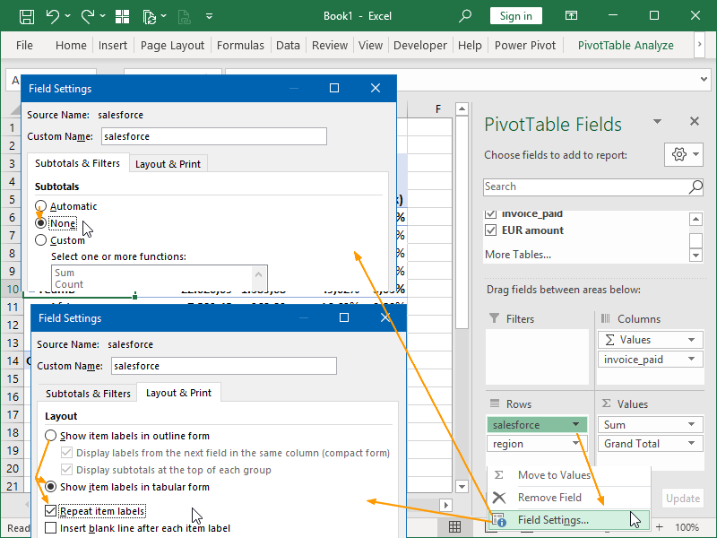
If we apply changes to this particular filed highlighted here, our pivot table will now look like this:
Pivot Table Fields: Filters
We can move already used or previously unused fields to Filters:
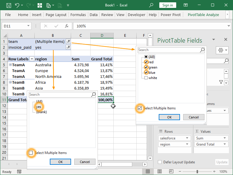
We can filter either by selecting a single item or by selecting multiple items:
We will have even more filtering options available if we apply filters directly on rows (or columns):
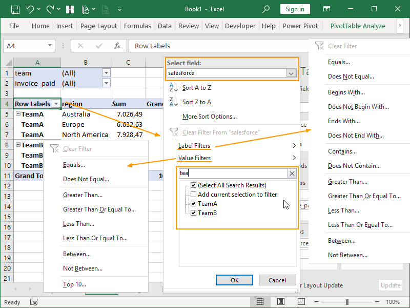
We can either filter directly from the pop-up window (those are Label Filters), or we use the Label Filters command for more options.
We can also apply value filters—those are also applied to the selected field we are filtering. For example, given that we are filtering the field salesforce, we can apply a filter that shows us only teams with the sum of values greater than the certain amount.
Sorting is also available here:
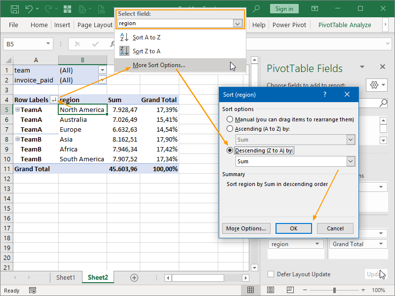
By positioning ourselves in the selected field or selecting that field from the drop-down menu, we can sort that field.
Not only that, but we can also sort that field by values.
As shown in this example, we are sorting the region field by Sum values in descending order.
Calculated Items & Calculated Fields
Calculated items are created by applying formulas onto items already existing in source columns.
If we position ourselves into a Pivot Table row or a column, the Insert Calculated Item option will become available:
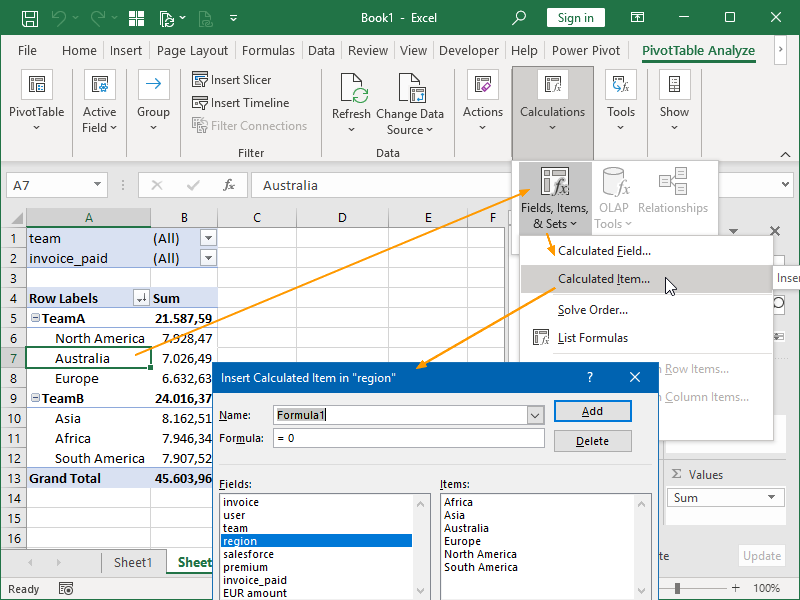
For example, we can create a new America item from North and South America:
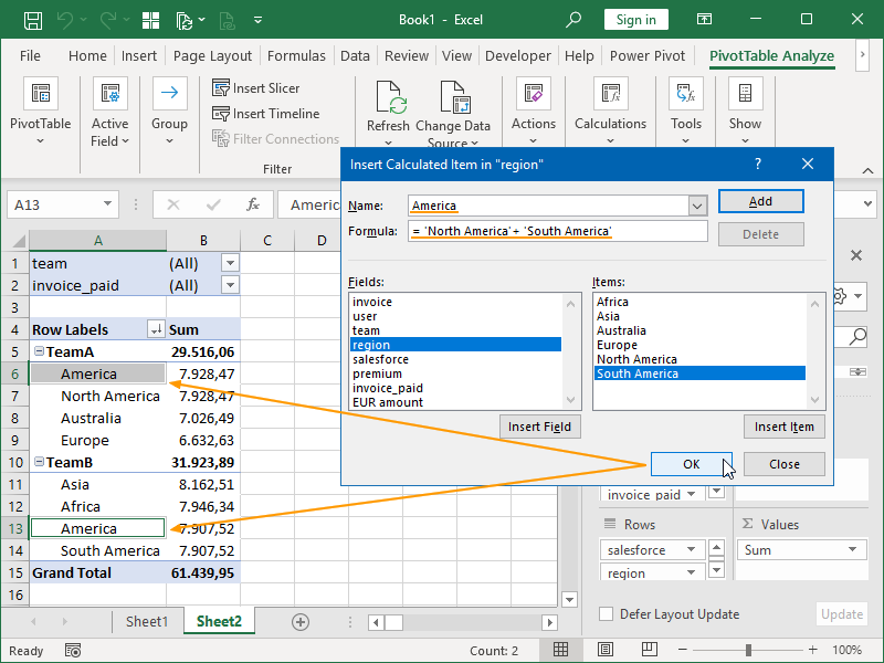
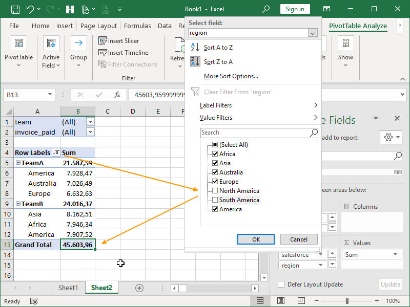
However, those values are by default duplicated now, and we have to filter out North and South America in order for our totals to be correct:
We can use Calculated Fields to perform basic calculations on existing columns containing values.
We can position ourselves anywhere in a Pivot Table, and the option to Insert Calculated Field will be available. In the next example, we will calculate a commission amount charged against our invoices:

We can also perform basic calculations with multiple (existing in the source data or calculated) columns. In the next example, we will subtract calculated commissions from our invoices:
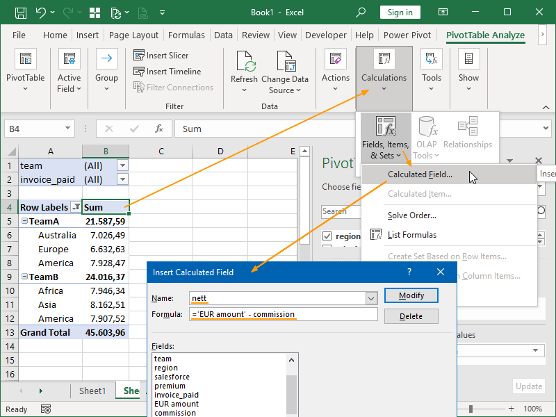
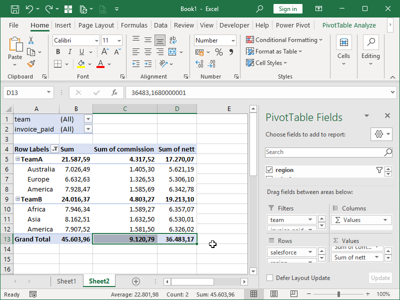
The result of those calculations will look like this:
Pivot Table Slicers
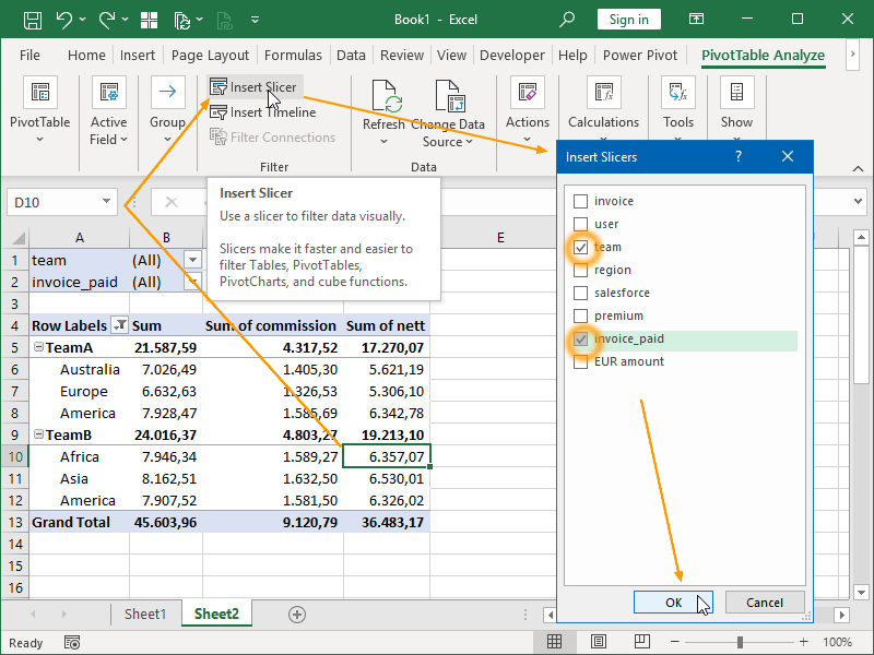
Slicers provide buttons that you can click in order to filter Pivot Tables. This quick filtering is especially useful when Pivot Tables are used as a reporting tool; other than enabling filtering, it also instantly visualizes what exactly is currently filtered.
We can insert one or more slicers under PivotTable Analyze, Insert Slicer:
In the following example, no team is filtered out, but paid invoices are filtered out. I.e., we are showing only the data for unpaid invoices:
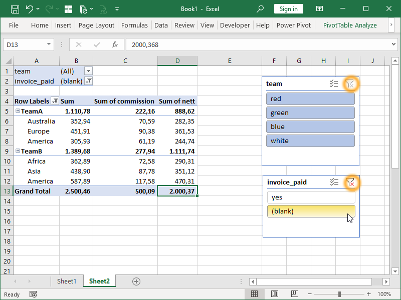
When a Slicer is active, a new tab, Slicer, also appears:
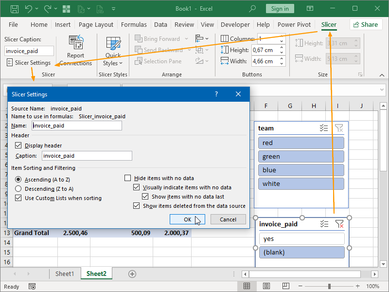
Here, we can further set up our slicers.
Pivot Table Timelines work much like Slicers, only they are intended for filtering dates.